MEEG Statistical Analysis Source Localization 2018 2019 ALISA

M/EEG Statistical Analysis & Source Localization 2018 -2019 ALISA LOOSEN & MATTHEW NOUR EXPERT: DR TIM TIERNEY METHODS FOR DUMMIES 2018/19

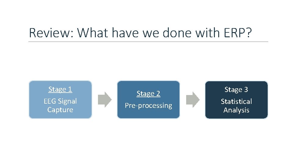
Review: What have we done with ERP? Stage 1 EEG Signal Capture Stage 2 Pre-processing Stage 3 Statistical Analysis

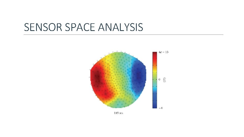
SENSOR SPACE ANALYSIS

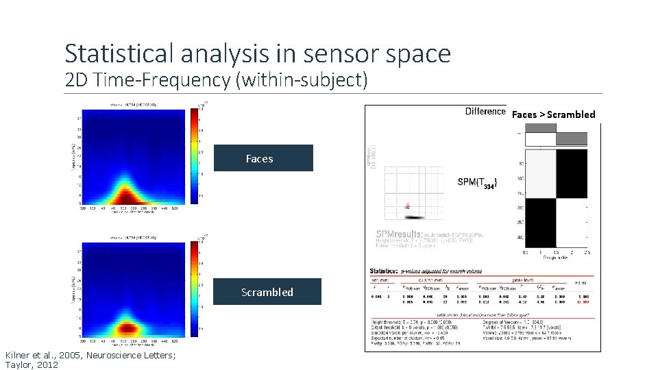
Statistical analysis in sensor space 2 D Time-Frequency (within-subject) Faces > Scrambled Faces Scrambled Kilner et al. , 2005, Neuroscience Letters; Taylor, 2012

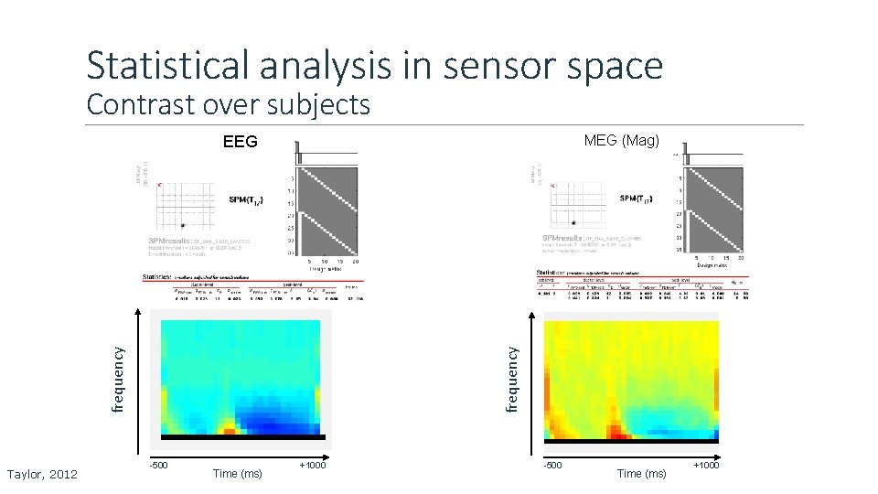
Statistical analysis in sensor space Contrast over subjects MEG (Mag) Taylor, 2012 frequency EEG -500 Time (ms) +1000

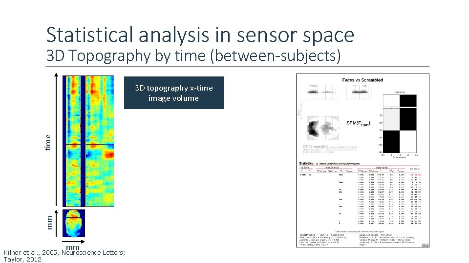
Statistical analysis in sensor space 3 D Topography by time (between-subjects) mm time 3 D topography x-time image volume mm Kilner et al. , 2005, Neuroscience Letters; Taylor, 2012

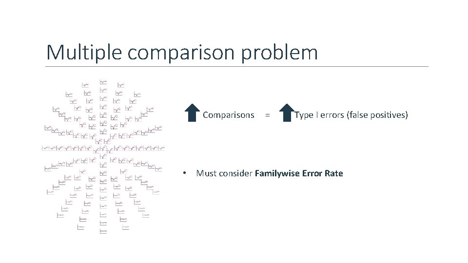
Multiple comparison problem Comparisons = Type I errors (false positives) • Must consider Familywise Error Rate

Statistical corrections • Bonferroni Correction • Too conservative • Random Field Theory is a method to correct for multiple statistical comparisons with N-dimensional spaces • Takes smoothness in the image into account • Implemented in SPM

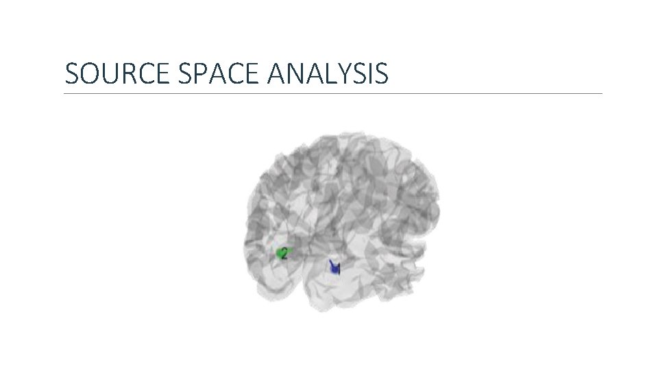
SOURCE SPACE ANALYSIS

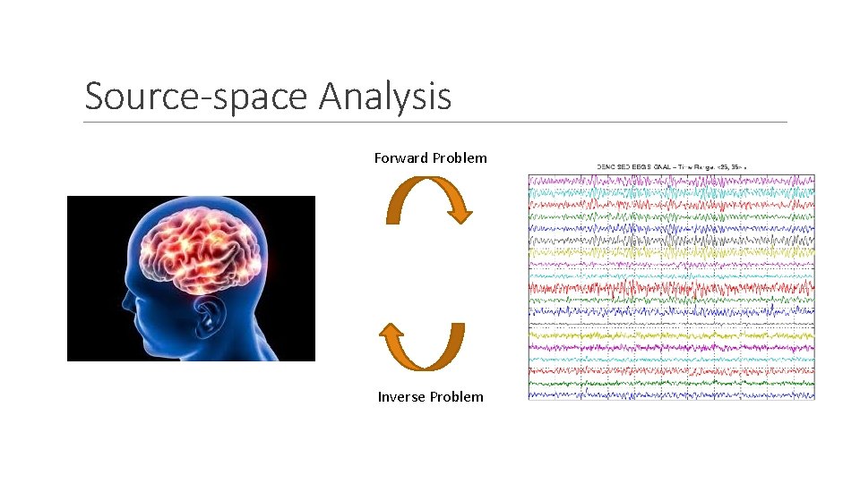
Source-space Analysis Forward Problem Inverse Problem

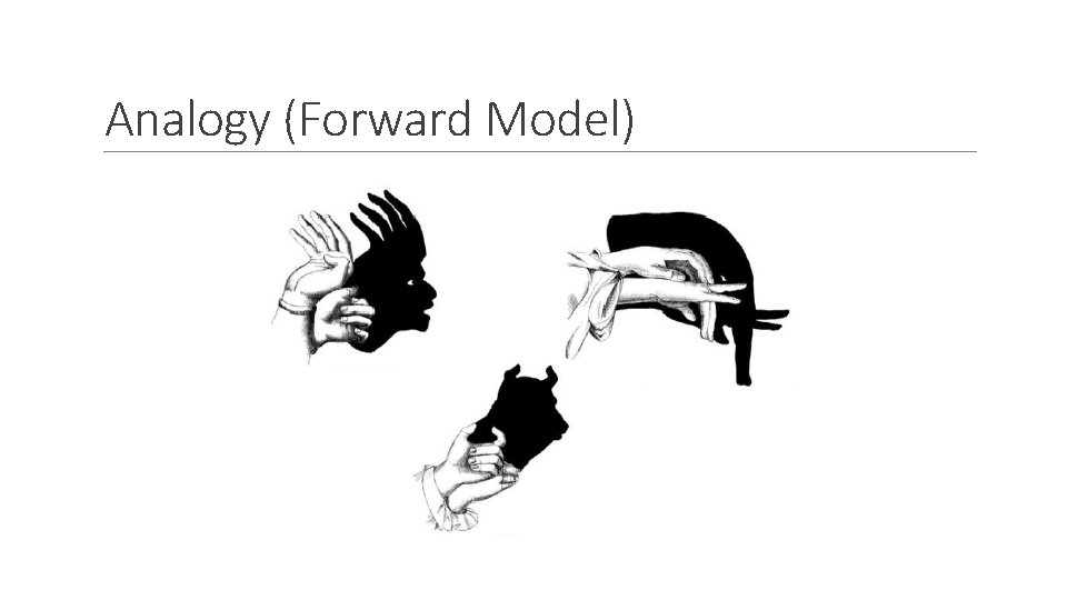
Analogy (Forward Model)

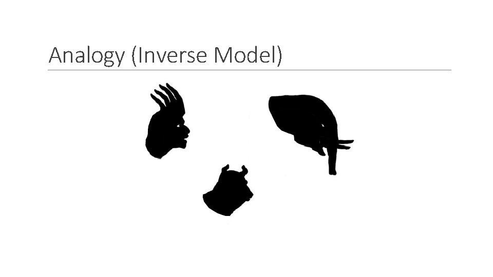
Analogy (Inverse Model)

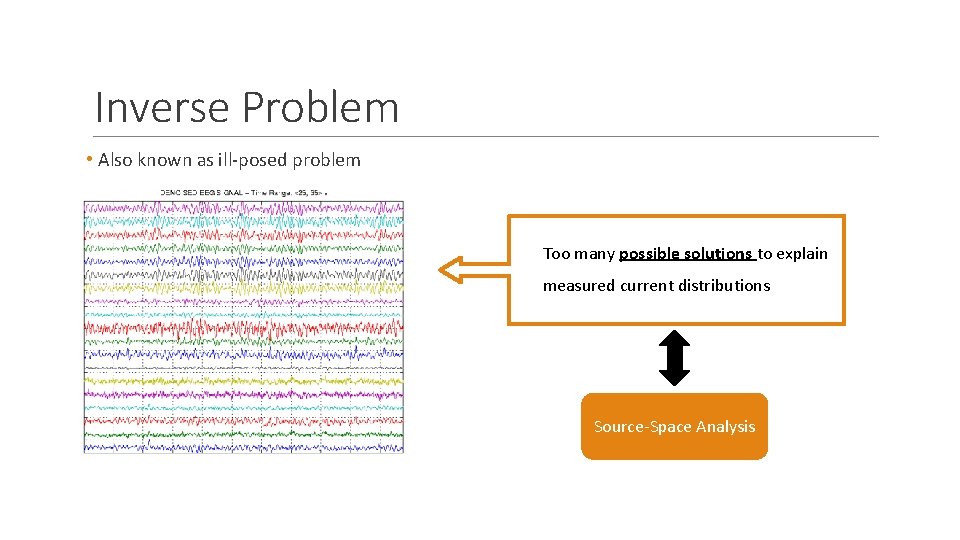
Inverse Problem • Also known as ill-posed problem Too many possible solutions to explain measured current distributions Source-Space Analysis

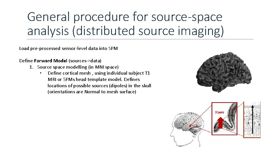
General procedure for source-space analysis (distributed source imaging) Load pre-processed sensor-level data into SPM Define Forward Model (sources->data) 1. Source space modelling (in MNI space) • Define cortical mesh , using individual subject T 1 MRI or SPMs head template model. Defines locations of possible sources (dipoles) in the skull (orientations are Normal to mesh surface) Dipole

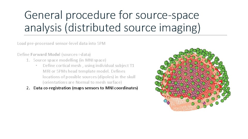
General procedure for source-space analysis (distributed source imaging) Load pre-processed sensor-level data into SPM Define Forward Model (sources->data) 1. Source space modelling (in MNI space) • Define cortical mesh , using individual subject T 1 MRI or SPMs head template model. Defines locations of possible sources (dipoles) in the skull (orientations are Normal to mesh surface) 2. Data co-registration (maps sensors to MNI coordinates)

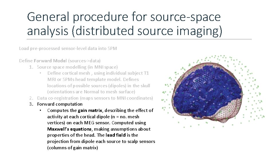
General procedure for source-space analysis (distributed source imaging) Load pre-processed sensor-level data into SPM Define Forward Model (sources->data) 1. Source space modelling (in MNI space) • Define cortical mesh , using individual subject T 1 MRI or SPMs head template model. Defines locations of possible sources (dipoles) in the skull (orientations are Normal to mesh surface) 2. Data co-registration (maps sensors to MNI coordinates) 3. Forward computation • Computes the gain matrix, describing the effect of activity at each cortical dipole (n = no. mesh vertices) on each MEG sensor. Computed using Maxwell’s equations, making assumptions about properties of the head. The lead field is the projection from dipole each source to scalp sensors (columns of gain matrix)

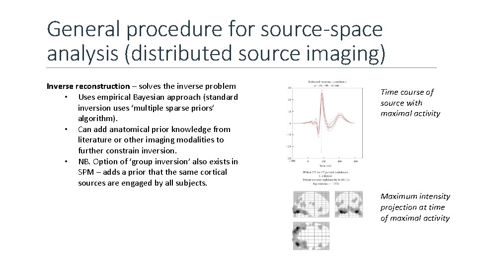
General procedure for source-space analysis (distributed source imaging) Inverse reconstruction – solves the inverse problem • Uses empirical Bayesian approach (standard inversion uses ‘multiple sparse priors’ algorithm). • Can add anatomical prior knowledge from literature or other imaging modalities to further constrain inversion. • NB. Option of ‘group inversion’ also exists in SPM – adds a prior that the same cortical sources are engaged by all subjects. Time course of source with maximal activity Maximum intensity projection at time of maximal activity

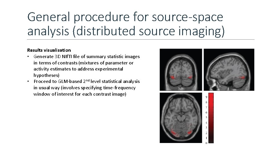
General procedure for source-space analysis (distributed source imaging) Results visualisation • Generate 3 D NIf. TI file of summary statistic images in terms of contrasts (mixtures of parameter or activity estimates to address experimental hypotheses) • Proceed to GLM-based 2 nd level statistical analysis in usual way (involves specifying time-frequency window of interest for each contrast image)

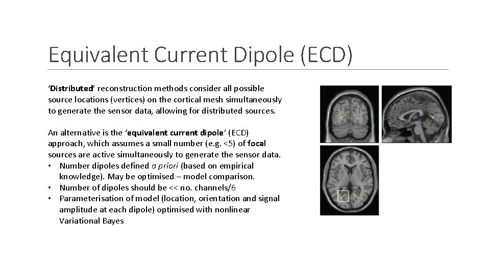
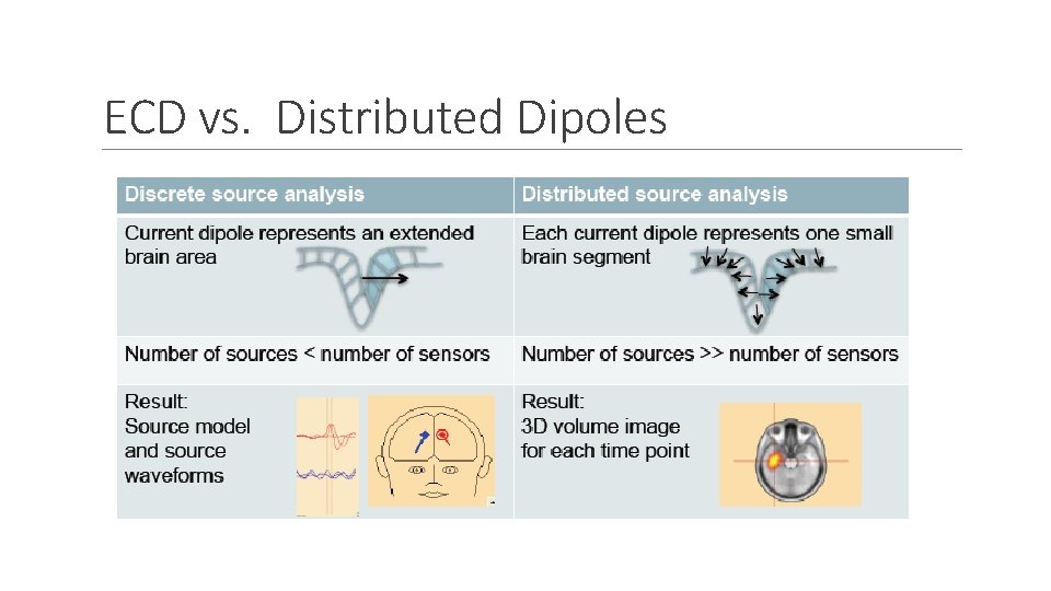
Equivalent Current Dipole (ECD) ‘Distributed’ reconstruction methods consider all possible source locations (vertices) on the cortical mesh simultaneously to generate the sensor data, allowing for distributed sources. An alternative is the ‘equivalent current dipole’ (ECD) approach, which assumes a small number (e. g. <5) of focal sources are active simultaneously to generate the sensor data. • Number dipoles defined a priori (based on empirical knowledge). May be optimised – model comparison. • Number of dipoles should be << no. channels/6 • Parameterisation of model (location, orientation and signal amplitude at each dipole) optimised with nonlinear Variational Bayes

ECD vs. Distributed Dipoles

Dynamic Causal Modelling (DCM) Augments the forward model • measured data are explained by a network of a few sources, which are dynamically coupled • model inversion optimises model parameters • Combines the spatial forward model (discussed previously) with a neurobiologicallyinformed temporal forward model. • Allows inference about connectivity architectures • As M/EEG data is highly time-resolved one can make inferences about e. g. synaptic time constants and receptor densities (impossible with DCM for f. MRI).

References • Kilner, J. and Friston, K. (2010). Topological inference for EEG and MEG. The Annals of Applied Statistics, 4(3), pp. 1272 -1290. • J. Kilner, S. J. Kiebel, and K. J. Friston. Applications of random field theory to electrophysiology. Neuroscience Letters, 374: 174 -178, 2005. • Litvak, V. , Mattout, J. , Kiebel, S. , Phillips, C. , Henson, R. , Kilner, J. , . . . & Penny, W. (2011). EEG and MEG data analysis in SPM 8. Computational intelligence and neuroscience, 2011. • Mf. D presentations from previous years • Lecture Slides from PSYCGC 11 Neuroimaging by Dr Leun Otten • Taylor, J. (2012). Statistical Analysis of M/EEG Sensor- and Source-Level Data.