MEEG Statistical analysis and source localisation Expert Vladimir

M/EEG: Statistical analysis and source localisation Expert: Vladimir Litvak Mathilde De Kerangal & Anne Löffler Methods for Dummies, March 2, 2016

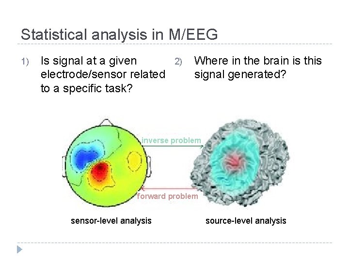
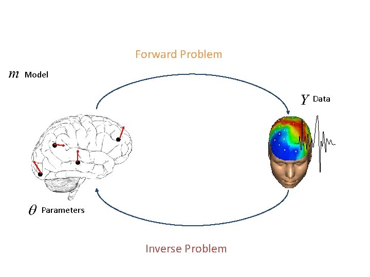
Statistical analysis in M/EEG 1) Is signal at a given electrode/sensor related to a specific task? 2) Where in the brain is this signal generated? inverse problem forward problem sensor-level analysis source-level analysis

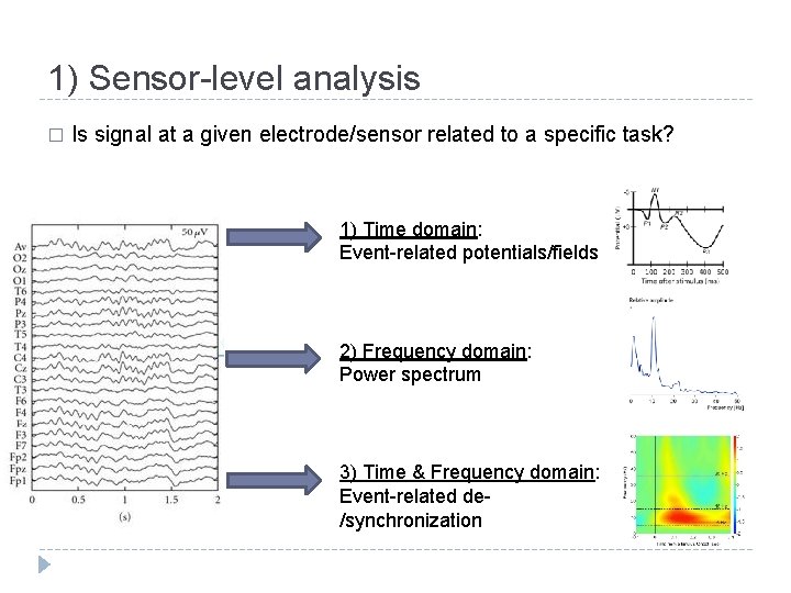
1) Sensor-level analysis � Is signal at a given electrode/sensor related to a specific task? 1) Time domain: Event-related potentials/fields 2) Frequency domain: Power spectrum 3) Time & Frequency domain: Event-related de/synchronization

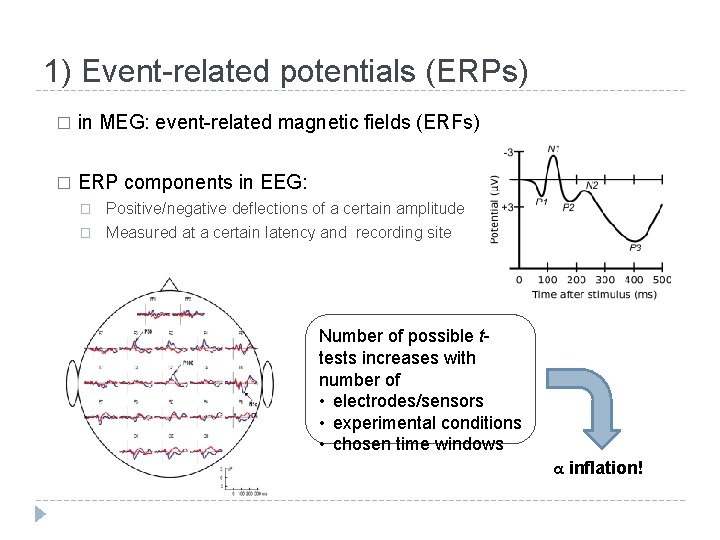
1) Event-related potentials (ERPs) � in MEG: event-related magnetic fields (ERFs) � ERP components in EEG: � Positive/negative deflections of a certain amplitude � Measured at a certain latency and recording site Number of possible ttests increases with number of • electrodes/sensors • experimental conditions • chosen time windows α inflation!

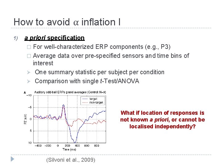
How to avoid α inflation I 1) a priori specification � For well-characterized ERP components (e. g. , P 3) � Average data over pre-specified sensors and time bins of interest Ø One summary statistic per subject per condition Ø Comparison with single t-Test/ANOVA What if location of responses is not known a priori, or cannot be localised independently? (Silvoni et al. , 2009)

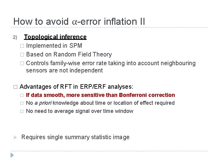
How to avoid α-error inflation II 2) Topological inference � Implemented in SPM � Based on Random Field Theory � Controls family-wise error rate taking into account neighbouring sensors are not independent � Advantages of RFT in ERP/ERF analyses: � � � Ø If data smooth, more sensitive than Bonferroni correction No a priori knowledge about time or location of effect required No need to average signal over time window Requires single summary statistic image

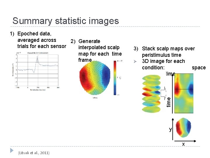
Summary statistic images 3) Stack scalp maps over peristimulus time Ø 3 D image for each condition: space x time 1) Epoched data, averaged across 2) Generate trials for each sensor interpolated scalp map for each time frame y x (Litvak et al. , 2011)

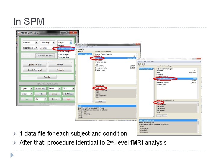
In SPM Ø Ø 1 data file for each subject and condition After that: procedure identical to 2 nd-level f. MRI analysis

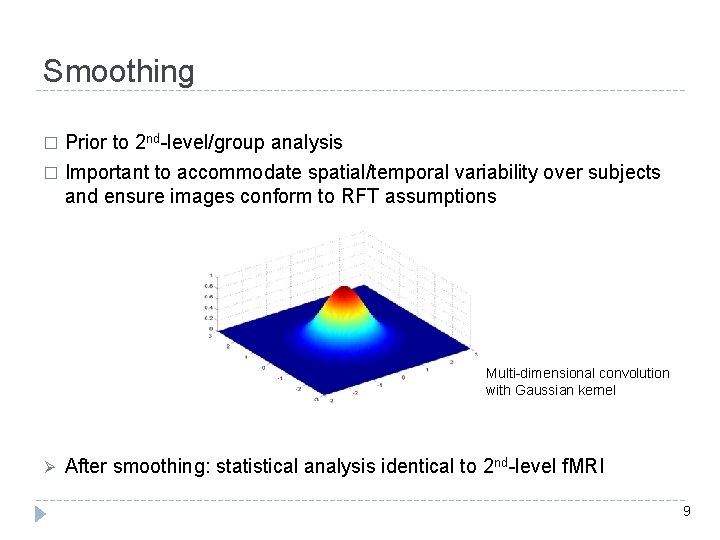
Smoothing Prior to 2 nd-level/group analysis � Important to accommodate spatial/temporal variability over subjects and ensure images conform to RFT assumptions � Multi-dimensional convolution with Gaussian kernel Ø After smoothing: statistical analysis identical to 2 nd-level f. MRI 9

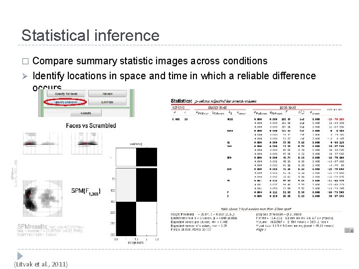
Statistical inference � Ø Compare summary statistic images across conditions Identify locations in space and time in which a reliable difference occurs (Litvak et al. , 2011)

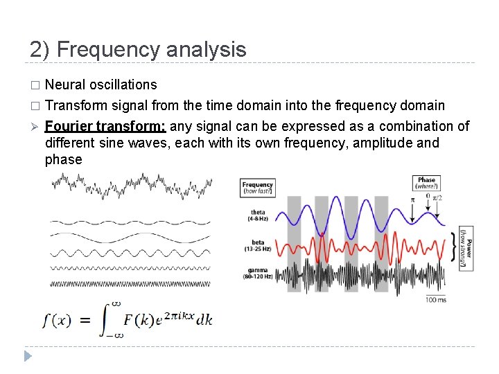
2) Frequency analysis Neural oscillations � Transform signal from the time domain into the frequency domain � Ø Fourier transform: any signal can be expressed as a combination of different sine waves, each with its own frequency, amplitude and phase

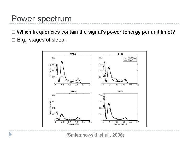
Power spectrum Which frequencies contain the signal’s power (energy per unit time)? � E. g. , stages of sleep: � (Smietanowski et al. , 2006)

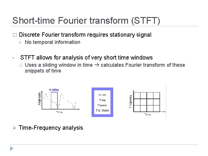
Short-time Fourier transform (STFT) � Discrete Fourier transform requires stationary signal Ø • STFT allows for analysis of very short time windows � Ø No temporal information Uses a sliding window in time calculates Fourier transform of these snippets of time Time-Frequency analysis

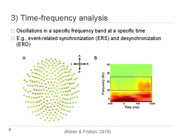
3) Time-frequency analysis Oscillations in a specific frequency band at a specific time � E. g. , event-related synchronization (ERS) and desynchronization (ERD) � (Kilner & Friston, 2010)

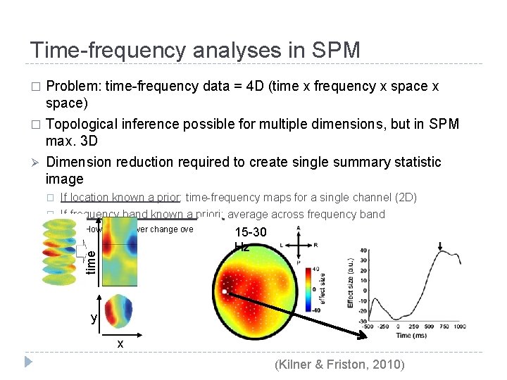
Time-frequency analyses in SPM � Problem: time-frequency data = 4 D (time x frequency x space) � Topological inference possible for multiple dimensions, but in SPM max. 3 D Dimension reduction required to create single summary statistic image � If location known a prior: time-frequency maps for a single channel (2 D) � If frequency band known a priori: average across frequency band Ø How does power change over space and 15 -30 time (3 D)? Hz time Ø y x (Kilner & Friston, 2010)

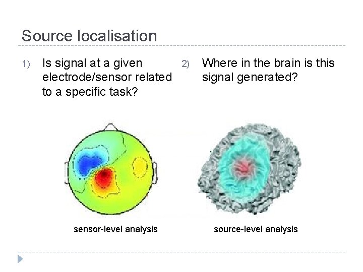
Source localisation 1) Is signal at a given electrode/sensor related to a specific task? 2) Where in the brain is this signal generated? inverse problem forward problem sensor-level analysis source-level analysis

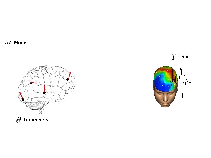
Model Data Parameters

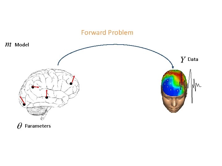
Forward Problem Model Data Parameters

Forward Problem Model Data Parameters Inverse Problem

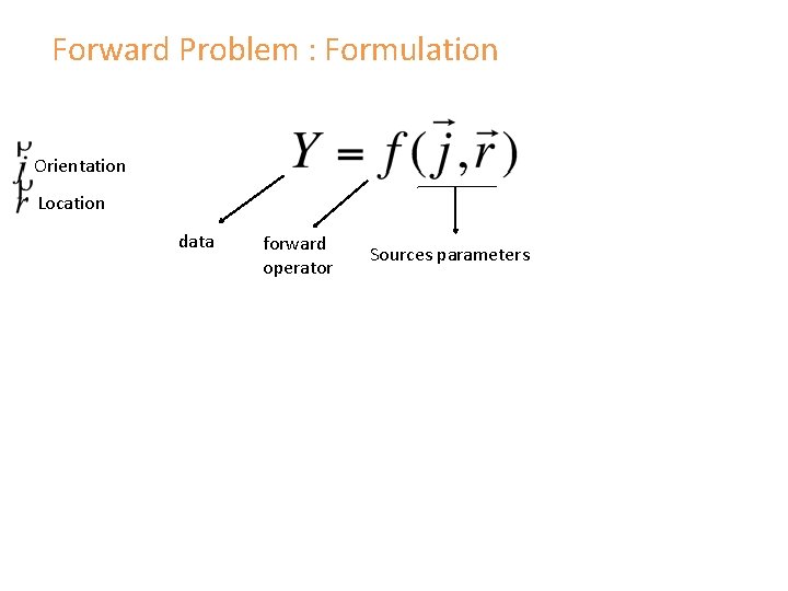
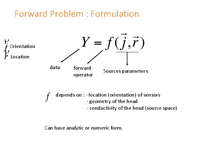
Forward Problem : Formulation Orientation Location data forward operator Sources parameters

Forward Problem : Formulation Orientation Location data forward operator Sources parameters depends on : - location (orientation) of sensors - geometry of the head - conductivity of the head (source space) Can have analytic or numeric form.

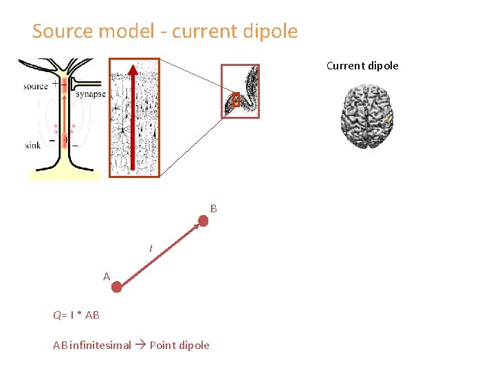
Source model - current dipole Current dipole B I A Q= I * AB AB infinitesimal Point dipole

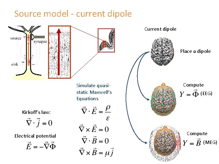
Source model - current dipole Current dipole Place a dipole Simulate quasistatic Maxwell’s Equations Compute (EEG) Kirkoff’s law: Electrical potential Compute (MEG)

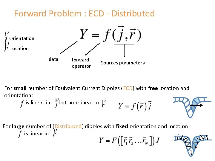
Forward Problem : ECD - Distributed Orientation Location data forward operator Sources parameters For small number of Equivalent Current Dipoles (ECD) with free location and orientation: is linear in but non-linear in For large number of (Distributed) dipoles with fixed orientation and location: is linear in

Equivalent current dipole : dipole fit 1. Select an initial guess for dipole location(s) 2. Calculate the smallest least-squares error between the measurement and the model data achievable by adjusting the dipole orientation(s) and amplitude(s) at this (/those) location(s). 3. If error is the same as in previous iteration step, STOP 4. Find a better candidate for the dipole location(s) 5. Go back to step 2 --> Very robust for one dipole

Equivalent current dipole : dipole fit Some problems… - A priori fixed number of sources considered. - Contraints on the dipole are difficult to include in the framework and noise cannot properly be taken into account. - Models with different ECDs cannot be compaired, except from goodness of fit which can be miseading, as adding dipoles to a model will necessariy improve the overall goodness of fit.

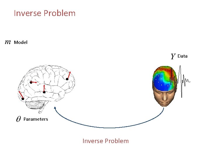
Inverse Problem Model Data Parameters Inverse Problem

Inverse Problem

Inverse Problem

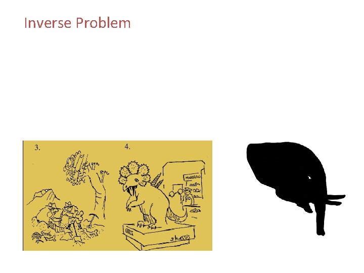
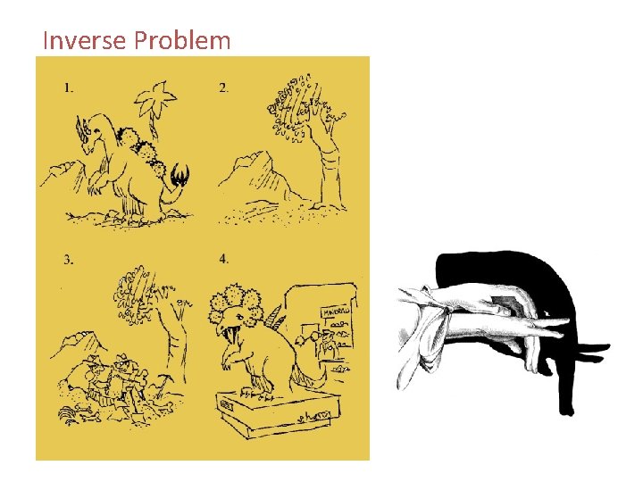
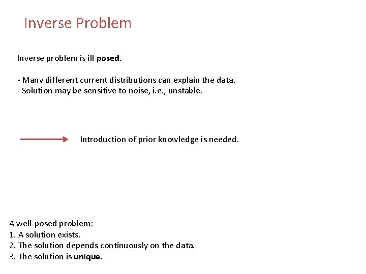
Inverse Problem Inverse problem is ill posed. - Many different current distributions can explain the data. - Solution may be sensitive to noise, i. e. , unstable. Introduction of prior knowledge is needed. A well-posed problem: 1. A solution exists. 2. The solution depends continuously on the data. 3. The solution is unique.

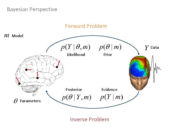
Bayesian Perspective Forward Problem Model Data Likelihood Posterior Prior Evidence Parameters Inverse Problem

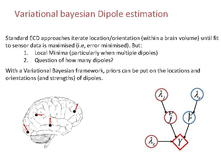
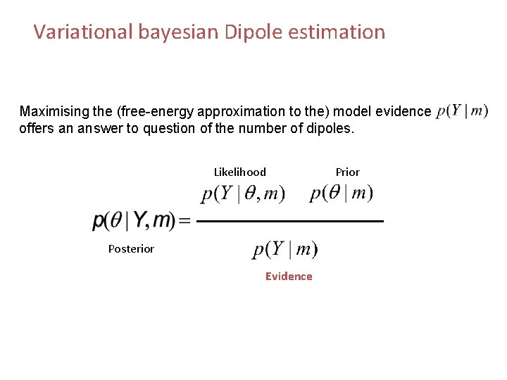
Variational bayesian Dipole estimation Standard ECD approaches iterate location/orientation (within a brain volume) until fit to sensor data is maximised (i. e, error minimised). But: 1. Local Minima (particularly when multiple dipoles) 2. Question of how many dipoles? With a Variational Bayesian framework, priors can be put on the locations and orientations (and strengths) of dipoles.

Variational bayesian Dipole estimation Maximising the (free-energy approximation to the) model evidence offers an answer to question of the number of dipoles. Likelihood Posterior Evidence Prior

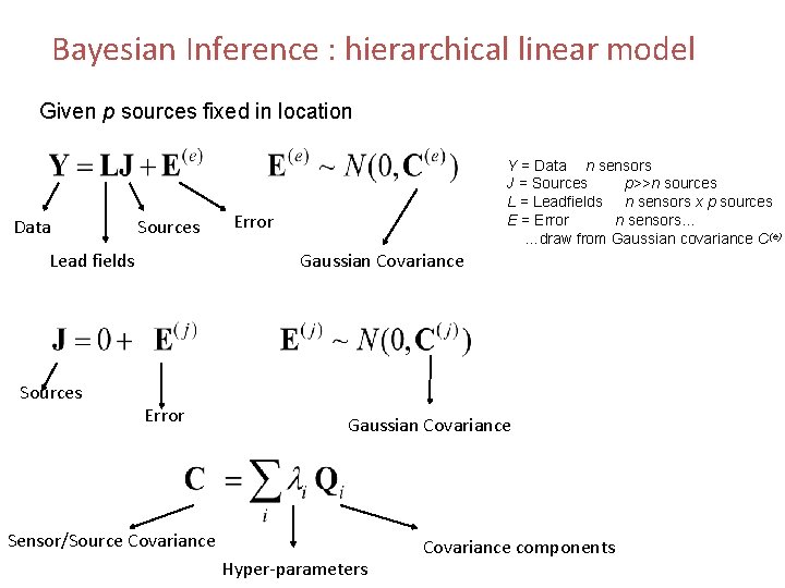
Bayesian Inference : hierarchical linear model Given p sources fixed in location Data Sources Error Gaussian Covariance Lead fields Sources Y = Data n sensors J = Sources p>>n sources L = Leadfields n sensors x p sources E = Error n sensors… …draw from Gaussian covariance C(e) Error Gaussian Covariance Sensor/Source Covariance Hyper-parameters Covariance components

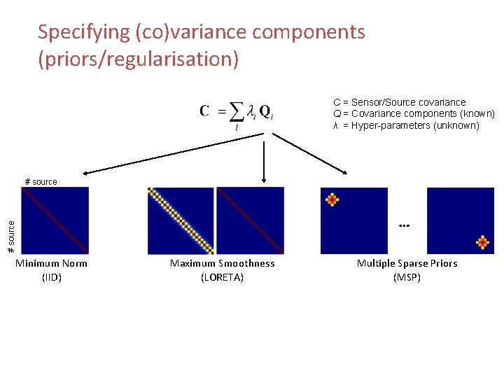
Specifying (co)variance components (priors/regularisation) C = Sensor/Source covariance Q = Covariance components (known) λ = Hyper-parameters (unknown) # source … Minimum Norm (IID) Maximum Smoothness (LORETA) Multiple Sparse Priors (MSP)

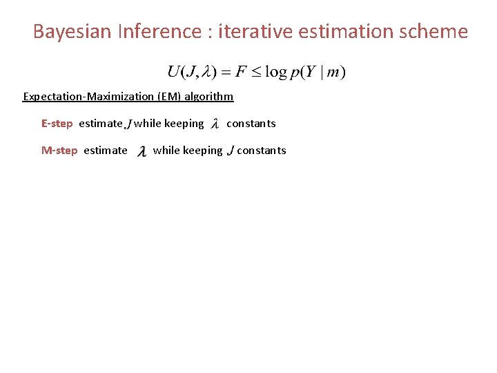
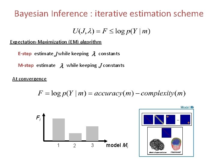
Bayesian Inference : iterative estimation scheme Expectation-Maximization (EM) algorithm E-step estimate while keeping M-step estimate while keeping constants

Bayesian Inference : iterative estimation scheme Expectation-Maximization (EM) algorithm E-step estimate while keeping M-step estimate constants while keeping constants At convergence Fi 1 2 3 model Mi

Inverse Problem DCM Dynamic Causal Modelling (DCM) can be seen as a source localisation (inverse) method that includes temporal constraints on the source activities. But this will be for another session…

Thank you for your attention! And a big thank you to our expert Vladimir Litvak!

References Kilner, J. M. , & Friston, K. J. (2010). Topological inference for EEG and MEG. The Annals of Applied Statistics, 1272 -1290. Litvak, V. , Mattout, J. , Kiebel, S. , Phillips, C. , Henson, R. , Kilner, J. , . . . & Penny, W. (2011). EEG and MEG data analysis in SPM 8. Computational intelligence and neuroscience, 2011. Mf. D presentations from previous years http: //imaging. mrc-cbu. cam. ac. uk/meg/Intro. EEGMEG#generalanalysis http: //www. timelycost. eu/sites/default/files/ppts/2 nd. Tr. Sc/Niko%20 Busch%20%20 Time%20 frequency%20 analysis%20 of%20 EEG%20 data. pdf http: //www. fil. ion. ucl. ac. uk/spm/course/ --> Presentation of Rick Henson SPM Course : Slides of Jeremie Mattout and Christophe Philip Oct 2008