LSP 121 Statistics That Deceive Simpsons Paradox It

Simpson’s Paradox • It is well accepted knowledge that the larger the data set,

Example: Simpson’s Paradox Baseball batting statistics for two players: First Half Second Half Total

Example Continued We weren’t told how many at bats each player had: First Half

Another Example Average college physics grades for students in an engineering program: Number of

Example continued In order to get better results, let’s combine our datasets. In particular,

Example continued Average college physics grades for students who took high school physics: Engineering

The Problem • Two problems with combining the data – There was a larger

Slides: 8

Download presentation

LSP 121 Statistics That Deceive

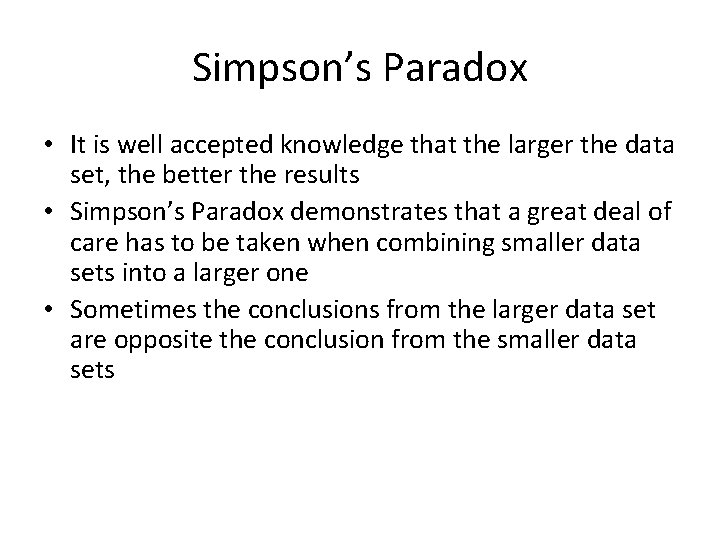
Simpson’s Paradox • It is well accepted knowledge that the larger the data set, the better the results • Simpson’s Paradox demonstrates that a great deal of care has to be taken when combining smaller data sets into a larger one • Sometimes the conclusions from the larger data set are opposite the conclusion from the smaller data sets

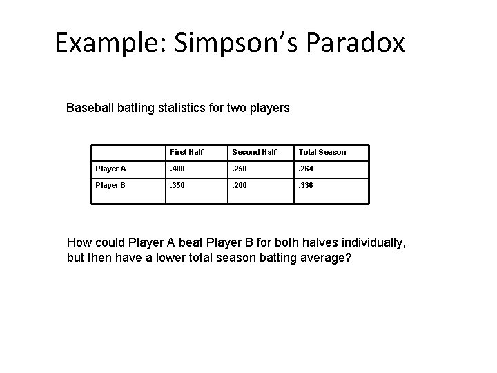
Example: Simpson’s Paradox Baseball batting statistics for two players: First Half Second Half Total Season Player A . 400 . 250 . 264 Player B . 350 . 200 . 336 How could Player A beat Player B for both halves individually, but then have a lower total season batting average?

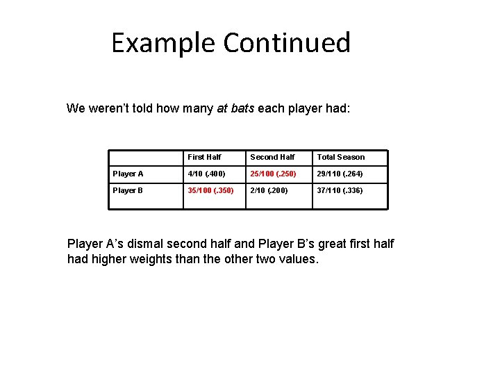
Example Continued We weren’t told how many at bats each player had: First Half Second Half Total Season Player A 4/10 (. 400) 25/100 (. 250) 29/110 (. 264) Player B 35/100 (. 350) 2/10 (. 200) 37/110 (. 336) Player A’s dismal second half and Player B’s great first half had higher weights than the other two values.

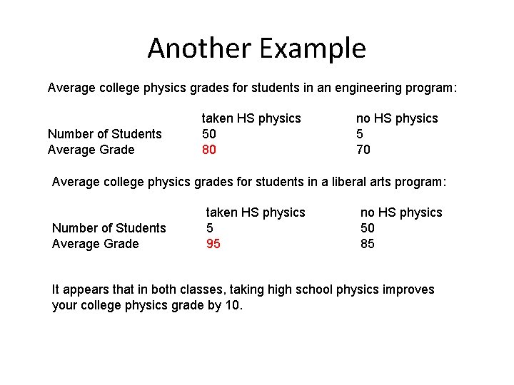
Another Example Average college physics grades for students in an engineering program: Number of Students Average Grade taken HS physics 50 80 no HS physics 5 70 Average college physics grades for students in a liberal arts program: Number of Students Average Grade taken HS physics 5 95 no HS physics 50 85 It appears that in both classes, taking high school physics improves your college physics grade by 10.

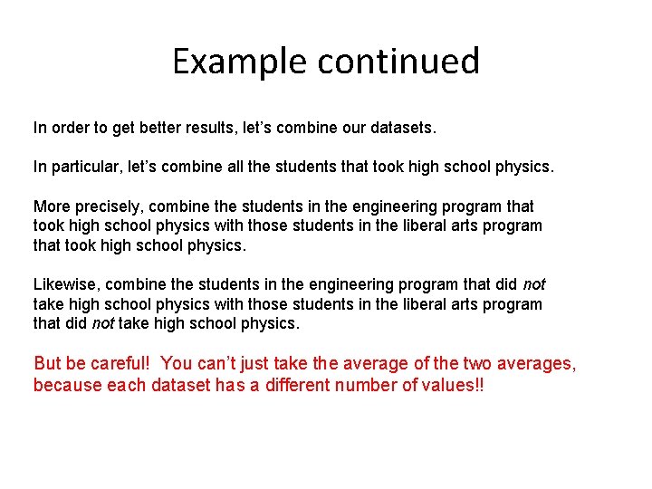
Example continued In order to get better results, let’s combine our datasets. In particular, let’s combine all the students that took high school physics. More precisely, combine the students in the engineering program that took high school physics with those students in the liberal arts program that took high school physics. Likewise, combine the students in the engineering program that did not take high school physics with those students in the liberal arts program that did not take high school physics. But be careful! You can’t just take the average of the two averages, because each dataset has a different number of values!!

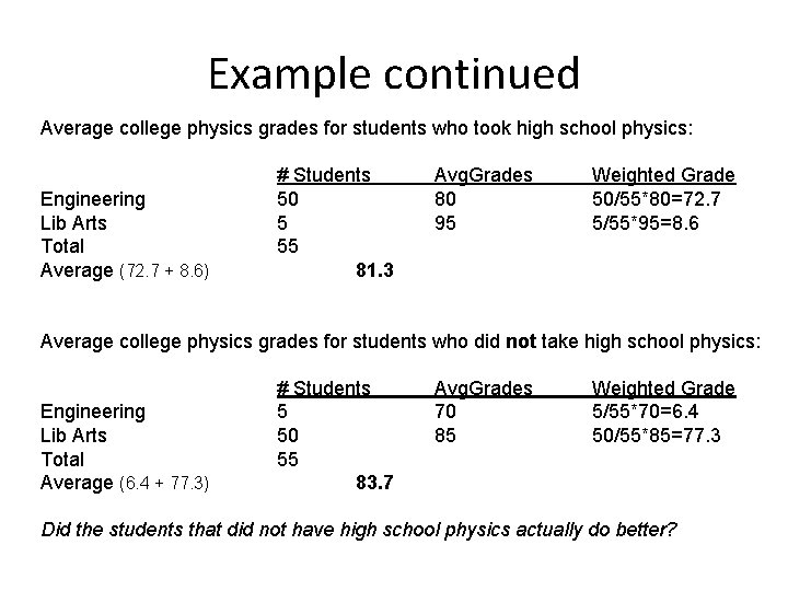
Example continued Average college physics grades for students who took high school physics: Engineering Lib Arts Total Average (72. 7 + 8. 6) # Students 50 5 55 81. 3 Avg. Grades 80 95 Weighted Grade 50/55*80=72. 7 5/55*95=8. 6 Average college physics grades for students who did not take high school physics: Engineering Lib Arts Total Average (6. 4 + 77. 3) # Students 5 50 55 83. 7 Avg. Grades 70 85 Weighted Grade 5/55*70=6. 4 50/55*85=77. 3 Did the students that did not have high school physics actually do better?

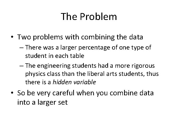
The Problem • Two problems with combining the data – There was a larger percentage of one type of student in each table – The engineering students had a more rigorous physics class than the liberal arts students, thus there is a hidden variable • So be very careful when you combine data into a larger set