Lecture 9 CS 3516 These slides are generated

Lecture 9 CS 3516: These slides are generated from those made available by the authors of our text. Computer Networking: A Top Down Approach 6 th edition Jim Kurose, Keith Ross Addison-Wesley March 2012 Introduction 1 -1

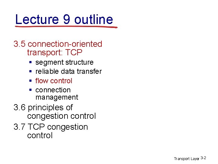
Lecture 9 outline 3. 5 connection-oriented transport: TCP § § segment structure reliable data transfer flow control connection management 3. 6 principles of congestion control 3. 7 TCP congestion control Transport Layer 3 -2

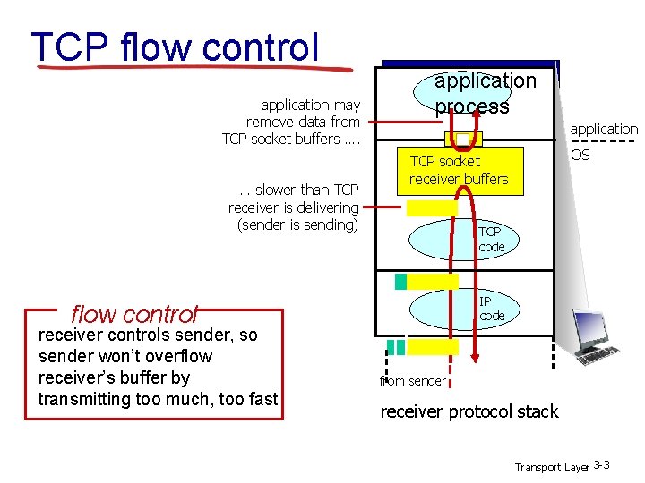
TCP flow control application may remove data from TCP socket buffers …. … slower than TCP receiver is delivering (sender is sending) application process application TCP code IP code flow control receiver controls sender, so sender won’t overflow receiver’s buffer by transmitting too much, too fast OS TCP socket receiver buffers from sender receiver protocol stack Transport Layer 3 -3

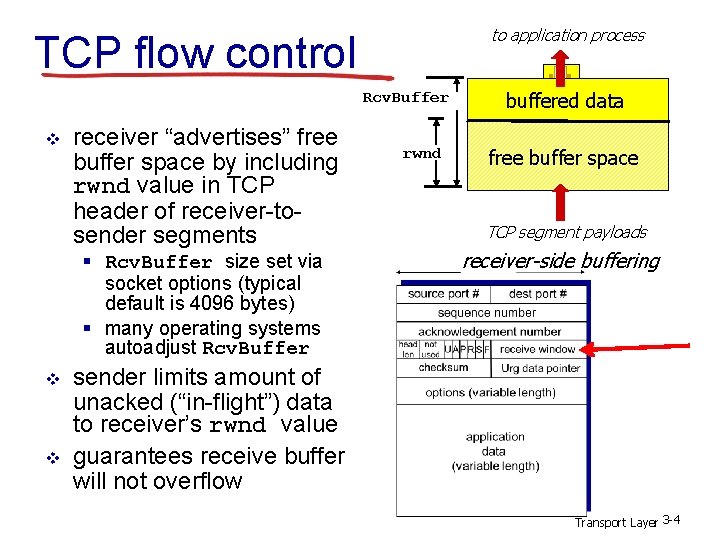
to application process TCP flow control Rcv. Buffer v receiver “advertises” free buffer space by including rwnd value in TCP header of receiver-tosender segments § Rcv. Buffer size set via socket options (typical default is 4096 bytes) § many operating systems autoadjust Rcv. Buffer v v rwnd buffered data free buffer space TCP segment payloads receiver-side buffering sender limits amount of unacked (“in-flight”) data to receiver’s rwnd value guarantees receive buffer will not overflow Transport Layer 3 -4

Lecture 9 outline 3. 5 connection-oriented transport: TCP § § segment structure reliable data transfer flow control connection management 3. 6 principles of congestion control 3. 7 TCP congestion control Transport Layer 3 -5

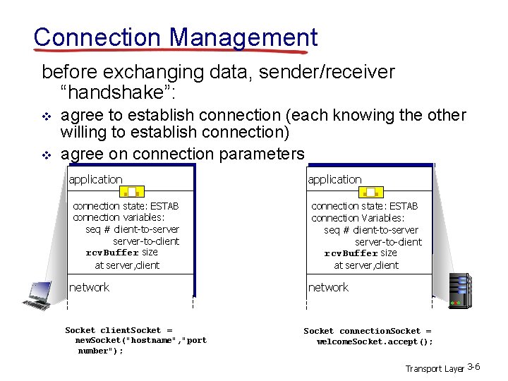
Connection Management before exchanging data, sender/receiver “handshake”: v v agree to establish connection (each knowing the other willing to establish connection) agree on connection parameters application connection state: ESTAB connection variables: seq # client-to-server-to-client rcv. Buffer size at server, client network Socket client. Socket = new. Socket("hostname", "port number"); application connection state: ESTAB connection Variables: seq # client-to-server-to-client rcv. Buffer size at server, client network Socket connection. Socket = welcome. Socket. accept(); Transport Layer 3 -6

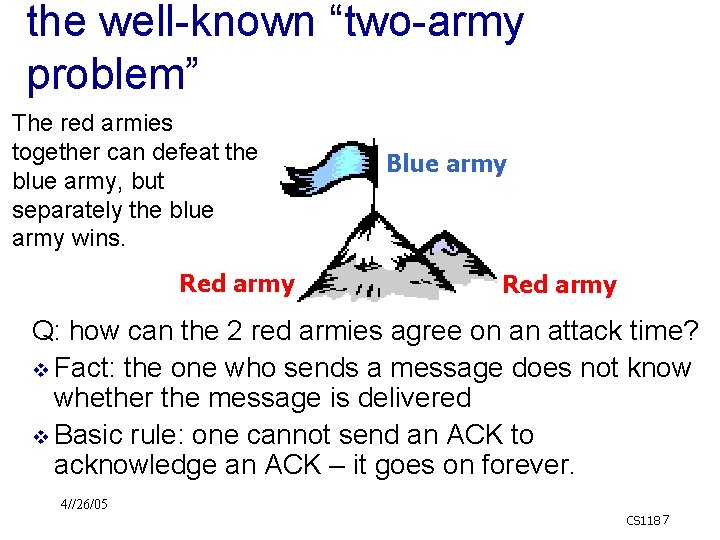
the well-known “two-army problem” The red armies together can defeat the blue army, but separately the blue army wins. Red army Blue army Red army Q: how can the 2 red armies agree on an attack time? v Fact: the one who sends a message does not know whether the message is delivered v Basic rule: one cannot send an ACK to acknowledge an ACK – it goes on forever. 4//26/05 CS 118 7

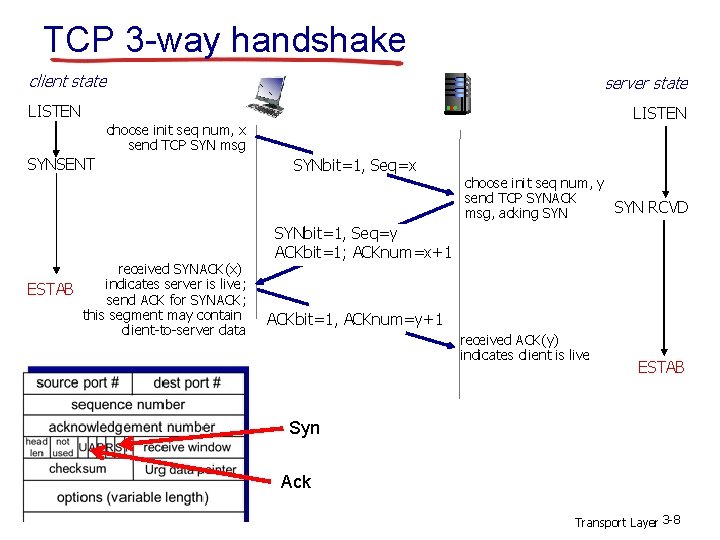
TCP 3 -way handshake client state server state LISTEN choose init seq num, x send TCP SYN msg SYNSENT received SYNACK(x) indicates server is live; ESTAB send ACK for SYNACK; this segment may contain client-to-server data SYNbit=1, Seq=x choose init seq num, y send TCP SYNACK SYN RCVD msg, acking SYNbit=1, Seq=y ACKbit=1; ACKnum=x+1 ACKbit=1, ACKnum=y+1 received ACK(y) indicates client is live ESTAB Syn Ack Transport Layer 3 -8

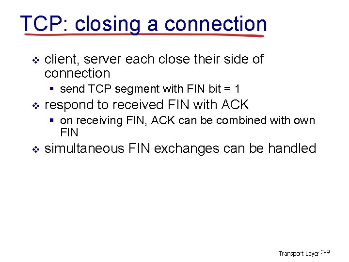
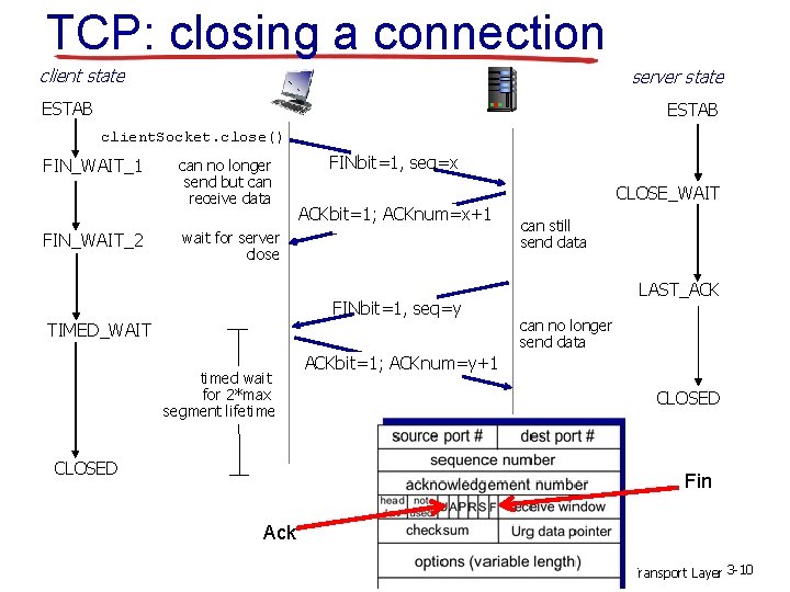
TCP: closing a connection v client, server each close their side of connection § send TCP segment with FIN bit = 1 v respond to received FIN with ACK § on receiving FIN, ACK can be combined with own FIN v simultaneous FIN exchanges can be handled Transport Layer 3 -9

TCP: closing a connection client state server state ESTAB client. Socket. close() FIN_WAIT_1 FIN_WAIT_2 can no longer send but can receive data FINbit=1, seq=x CLOSE_WAIT ACKbit=1; ACKnum=x+1 wait for server close FINbit=1, seq=y TIMED_WAIT timed wait for 2*max segment lifetime CLOSED can still send data LAST_ACK can no longer send data ACKbit=1; ACKnum=y+1 CLOSED Fin Ack Transport Layer 3 -10

Lecture 9 outline 3. 5 connection-oriented transport: TCP § § segment structure reliable data transfer flow control connection management 3. 6 principles of congestion control 3. 7 TCP congestion control Transport Layer 3 -11

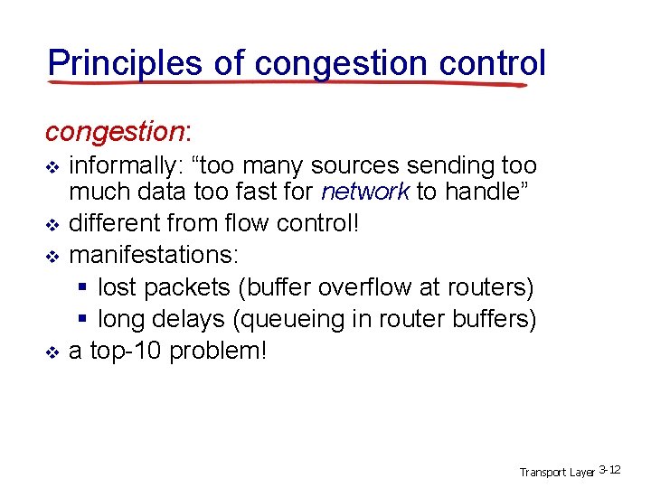
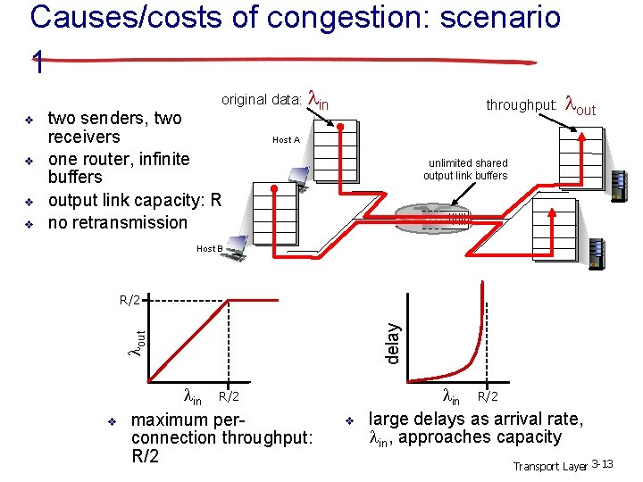
Principles of congestion control congestion: v v informally: “too many sources sending too much data too fast for network to handle” different from flow control! manifestations: § lost packets (buffer overflow at routers) § long delays (queueing in router buffers) a top-10 problem! Transport Layer 3 -12

Causes/costs of congestion: scenario 1 original data: lin v v lout Host A unlimited shared output link buffers Host B R/2 delay v two senders, two receivers one router, infinite buffers output link capacity: R no retransmission lout v throughput: v lin R/2 maximum perconnection throughput: R/2 v lin R/2 large delays as arrival rate, lin, approaches capacity Transport Layer 3 -13

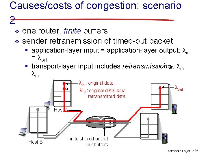
Causes/costs of congestion: scenario 2 v v one router, finite buffers sender retransmission of timed-out packet § application-layer input = application-layer output: lin = lout ‘ : l § transport-layer input includes retransmissions in lin : original data l'in: original data, plus lout retransmitted data Host A Host B finite shared output link buffers Transport Layer 3 -14

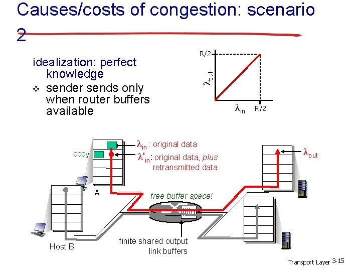
Causes/costs of congestion: scenario 2 R/2 lout idealization: perfect knowledge v sender sends only when router buffers available lin : original data l'in: original data, plus copy R/2 lout retransmitted data A Host B free buffer space! finite shared output link buffers Transport Layer 3 -15

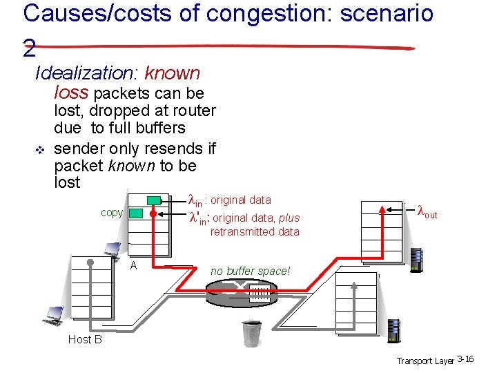
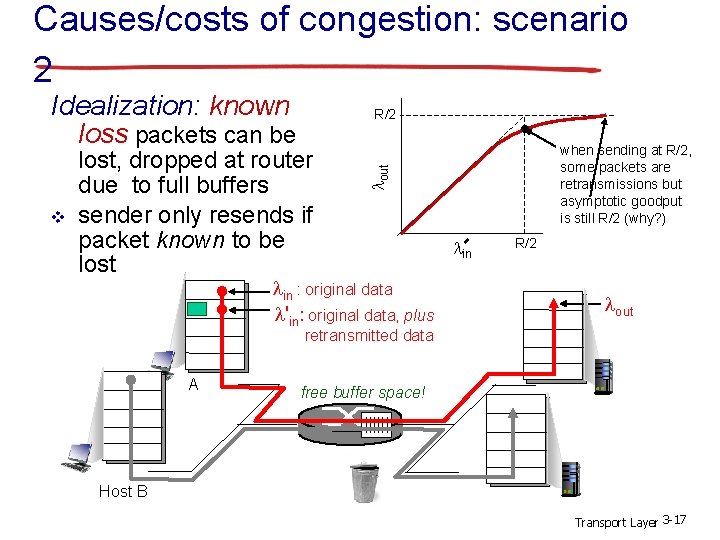
Causes/costs of congestion: scenario 2 Idealization: known loss packets can be v lost, dropped at router due to full buffers sender only resends if packet known to be lost lin : original data l'in: original data, plus copy lout retransmitted data A no buffer space! Host B Transport Layer 3 -16

Causes/costs of congestion: scenario 2 v R/2 lost, dropped at router due to full buffers sender only resends if packet known to be lost when sending at R/2, some packets are retransmissions but asymptotic goodput is still R/2 (why? ) lout Idealization: known loss packets can be lin : original data l'in: original data, plus lin R/2 lout retransmitted data A free buffer space! Host B Transport Layer 3 -17

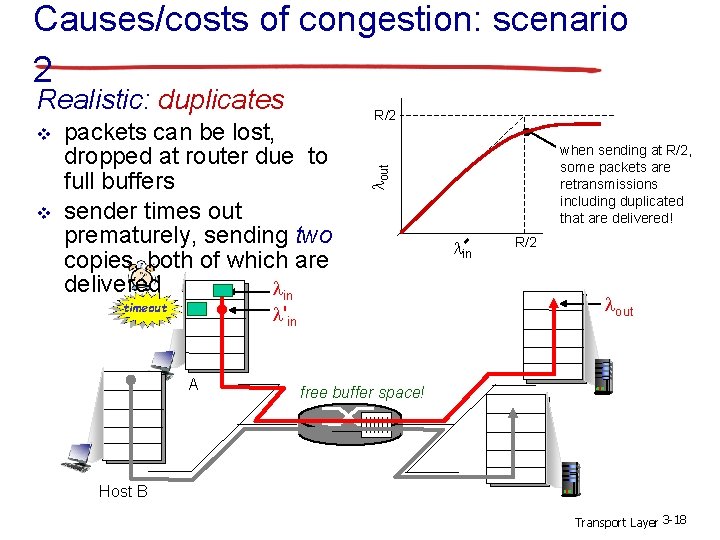
Causes/costs of congestion: scenario 2 v v packets can be lost, dropped at router due to full buffers sender times out prematurely, sending two copies, both of which are delivered lin timeout copy R/2 l'in A when sending at R/2, some packets are retransmissions including duplicated that are delivered! lout Realistic: duplicates lin R/2 lout free buffer space! Host B Transport Layer 3 -18

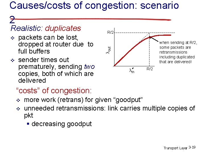
Causes/costs of congestion: scenario 2 v v packets can be lost, dropped at router due to full buffers sender times out prematurely, sending two copies, both of which are delivered R/2 when sending at R/2, some packets are retransmissions including duplicated that are delivered! lout Realistic: duplicates lin R/2 “costs” of congestion: v v more work (retrans) for given “goodput” unneeded retransmissions: link carries multiple copies of pkt § decreasing goodput Transport Layer 3 -19

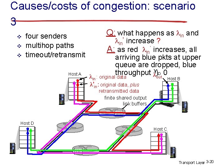
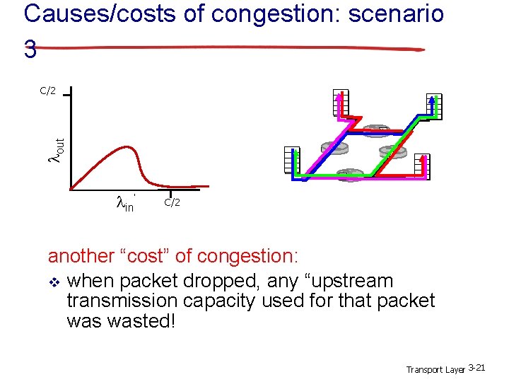
Causes/costs of congestion: scenario 3 v v v four senders multihop paths timeout/retransmit Host A Q: what happens as lin and lin’ increase ? A: as red lin’ increases, all arriving blue pkts at upper queue are dropped, blue throughput lg 0 out Host B lin : original data l'in: original data, plus retransmitted data finite shared output link buffers Host D Host C Transport Layer 3 -20

Causes/costs of congestion: scenario 3 lout C/2 lin’ C/2 another “cost” of congestion: v when packet dropped, any “upstream transmission capacity used for that packet wasted! Transport Layer 3 -21

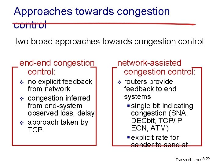
Approaches towards congestion control two broad approaches towards congestion control: end-end congestion control: v v v no explicit feedback from network congestion inferred from end-system observed loss, delay approach taken by TCP network-assisted congestion control: v routers provide feedback to end systems § single bit indicating congestion (SNA, DECbit, TCP/IP ECN, ATM) § explicit rate for sender to send at Transport Layer 3 -22

Lecture 9 outline 3. 5 connection-oriented transport: TCP § § segment structure reliable data transfer flow control connection management 4. 5 routing algorithms §link state §distance vector §hierarchical routing 3. 6 principles of congestion control 3. 7 TCP congestion control Transport Layer 3 -23

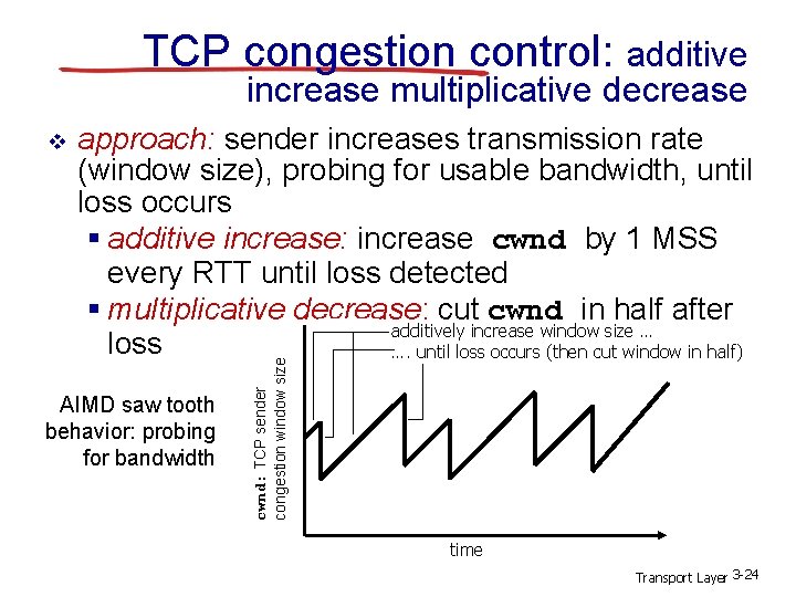
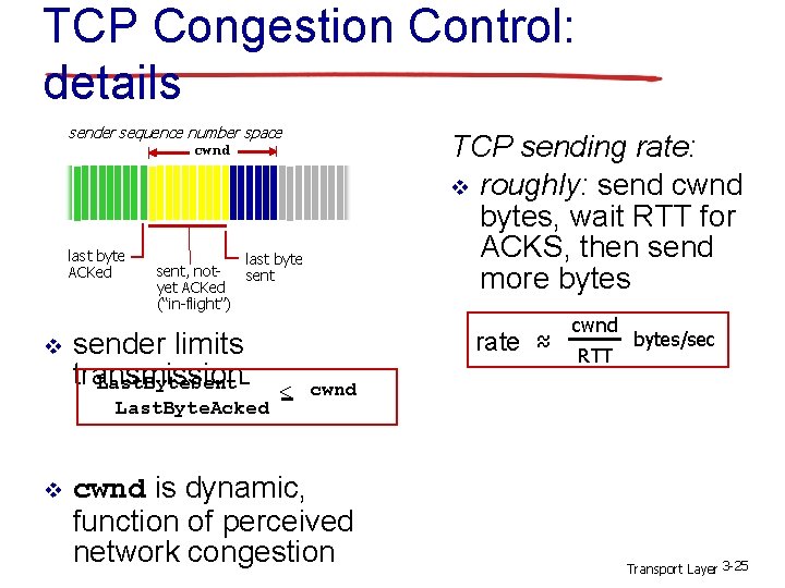
TCP congestion control: additive increase multiplicative decrease approach: sender increases transmission rate (window size), probing for usable bandwidth, until loss occurs § additive increase: increase cwnd by 1 MSS every RTT until loss detected § multiplicative decrease: cut cwnd in half after additively increase window size … loss …. until loss occurs (then cut window in half) AIMD saw tooth behavior: probing for bandwidth cwnd: TCP sender congestion window size v time Transport Layer 3 -24

TCP Congestion Control: details sender sequence number space cwnd last byte ACKed v last byte sent, notsent yet ACKed (“in-flight”) sender limits transmission: Last. Byte. Sent. Last. Byte. Acked v TCP sending rate: v roughly: send cwnd bytes, wait RTT for ACKS, then send more bytes rate ~ ~ cwnd RTT bytes/sec < cwnd is dynamic, function of perceived network congestion Transport Layer 3 -25

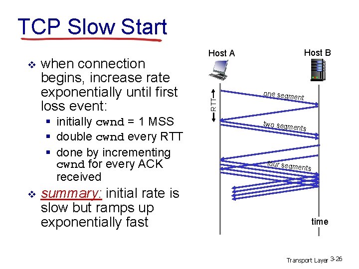
TCP Slow Start when connection begins, increase rate exponentially until first loss event: § initially cwnd = 1 MSS § double cwnd every RTT § done by incrementing cwnd for every ACK received v summary: initial rate is slow but ramps up exponentially fast RTT v Host B Host A one segm ent two segm ents four segm ents time Transport Layer 3 -26

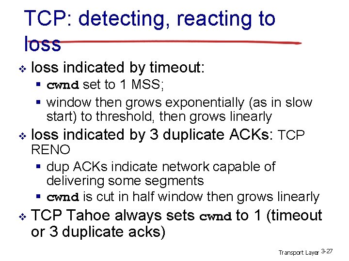
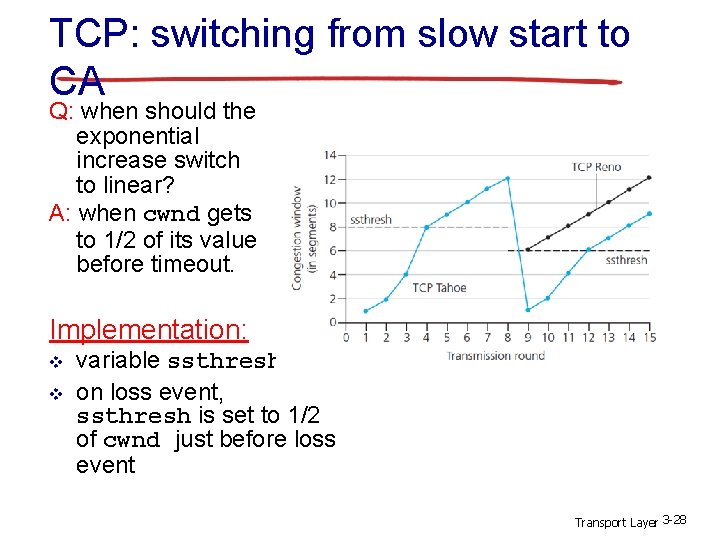
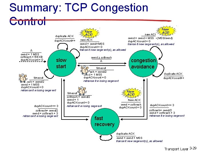
TCP: detecting, reacting to loss v loss indicated by timeout: § cwnd set to 1 MSS; § window then grows exponentially (as in slow start) to threshold, then grows linearly v loss indicated by 3 duplicate ACKs: TCP RENO § dup ACKs indicate network capable of delivering some segments § cwnd is cut in half window then grows linearly v TCP Tahoe always sets cwnd to 1 (timeout or 3 duplicate acks) Transport Layer 3 -27

TCP: switching from slow start to CA Q: when should the exponential increase switch to linear? A: when cwnd gets to 1/2 of its value before timeout. Implementation: v v variable ssthresh on loss event, ssthresh is set to 1/2 of cwnd just before loss event Transport Layer 3 -28

Summary: TCP Congestion Control duplicate ACK dup. ACKcount++ L cwnd = 1 MSS ssthresh = 64 KB dup. ACKcount = 0 slow start timeout ssthresh = cwnd/2 cwnd = 1 MSS dup. ACKcount = 0 retransmit missing segment dup. ACKcount == 3 ssthresh= cwnd/2 cwnd = ssthresh + 3 retransmit missing segment New ACK! new ACK cwnd = cwnd+MSS dup. ACKcount = 0 transmit new segment(s), as allowed cwnd > ssthresh L timeout ssthresh = cwnd/2 cwnd = 1 MSS dup. ACKcount = 0 retransmit missing segment timeout ssthresh = cwnd/2 cwnd = 1 dup. ACKcount = 0 retransmit missing segment . New ACK! new ACK cwnd = cwnd + MSS (MSS/cwnd) dup. ACKcount = 0 transmit new segment(s), as allowed congestion avoidance duplicate ACK dup. ACKcount++ New ACK! New ACK cwnd = ssthresh dup. ACKcount = 0 fast recovery dup. ACKcount == 3 ssthresh= cwnd/2 cwnd = ssthresh + 3 retransmit missing segment duplicate ACK cwnd = cwnd + MSS transmit new segment(s), as allowed Transport Layer 3 -29

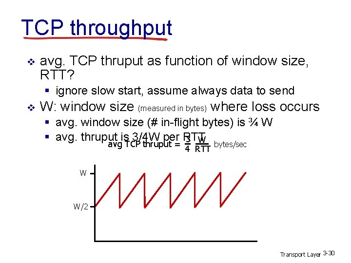
TCP throughput v avg. TCP thruput as function of window size, RTT? § ignore slow start, assume always data to send v W: window size (measured in bytes) where loss occurs § avg. window size (# in-flight bytes) is ¾ W § avg. thruput is 3/4 W per RTT 3 W avg TCP thruput = 4 RTT bytes/sec W W/2 Transport Layer 3 -30

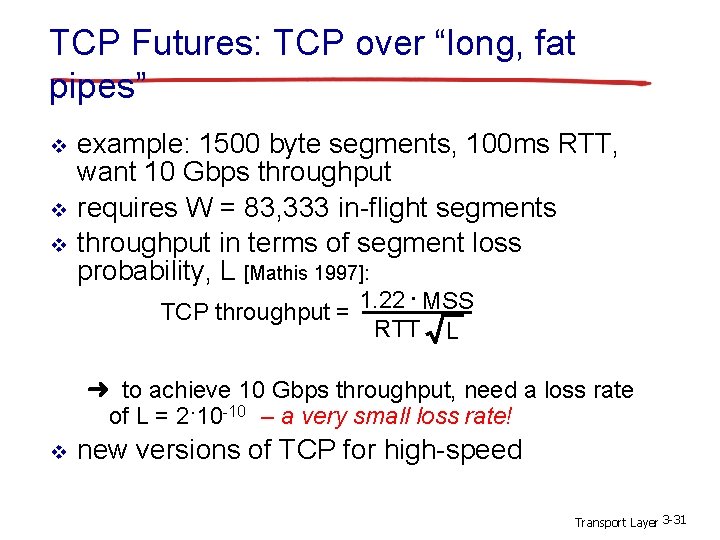
TCP Futures: TCP over “long, fat pipes” v v v example: 1500 byte segments, 100 ms RTT, want 10 Gbps throughput requires W = 83, 333 in-flight segments throughput in terms of segment loss probability, L [Mathis 1997]: 1. 22. MSS TCP throughput = RTT L ➜ to achieve 10 Gbps throughput, need a loss rate of L = 2·10 -10 – a very small loss rate! v new versions of TCP for high-speed Transport Layer 3 -31

Lecture 9 outline 3. 5 connection-oriented transport: TCP § § segment structure reliable data transfer flow control connection management 4. 5 routing algorithms §link state §distance vector §hierarchical routing 3. 6 principles of congestion control 3. 7 TCP congestion control Transport Layer 3 -32

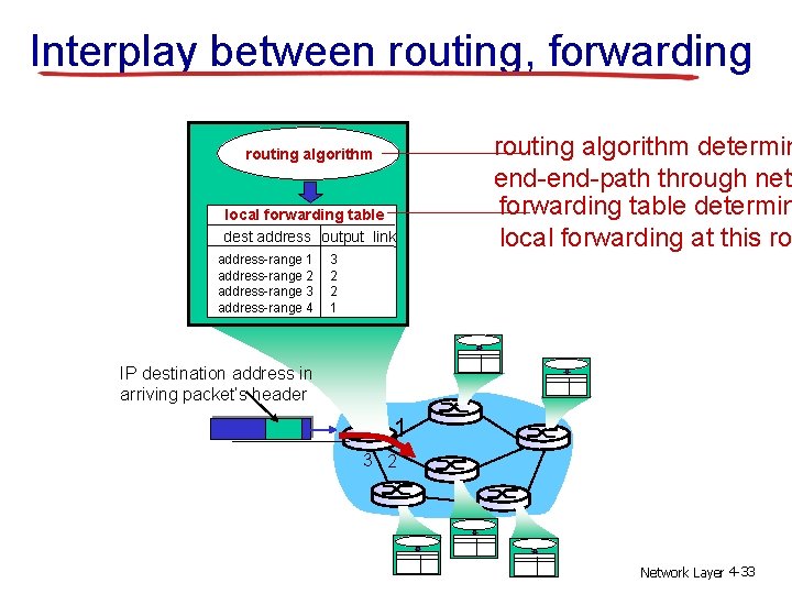
Interplay between routing, forwarding routing algorithm local forwarding table dest address output link address-range 1 address-range 2 address-range 3 address-range 4 routing algorithm determin end-path through netw forwarding table determin local forwarding at this ro 3 2 2 1 IP destination address in arriving packet’s header 1 3 2 Network Layer 4 -33

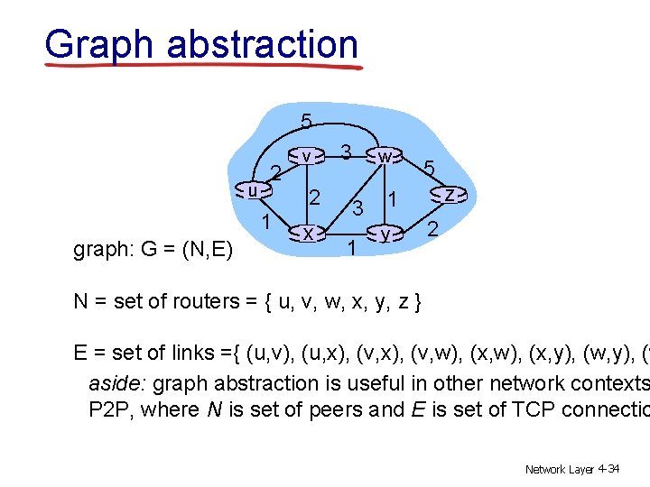
Graph abstraction 5 u 2 1 graph: G = (N, E) v 2 x 3 w 3 1 1 y 5 z 2 N = set of routers = { u, v, w, x, y, z } E = set of links ={ (u, v), (u, x), (v, w), (x, y), (w aside: graph abstraction is useful in other network contexts P 2 P, where N is set of peers and E is set of TCP connectio Network Layer 4 -34

Graph abstraction: costs 5 u 2 1 v 2 x 3 w 3 1 1 y c(x, x’) = cost of link (x, x’) e. g. , c(w, z) = 5 5 z 2 cost could always be 1, or inversely related to bandwidth, or inversely related to congestion cost of path (x 1, x 2, x 3, …, xp) = c(x 1, x 2) + c(x 2, x 3) + … + c(xp-1, xp) key question: what is the least-cost path between u and z ? routing algorithm: algorithm that finds that least cost path Network Layer 4 -35

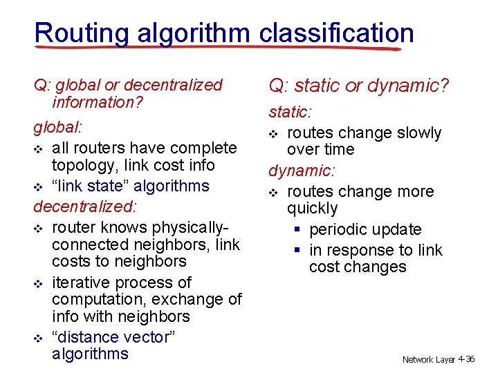
Routing algorithm classification Q: global or decentralized information? global: v all routers have complete topology, link cost info v “link state” algorithms decentralized: v router knows physicallyconnected neighbors, link costs to neighbors v iterative process of computation, exchange of info with neighbors v “distance vector” algorithms Q: static or dynamic? static: v routes change slowly over time dynamic: v routes change more quickly § periodic update § in response to link cost changes Network Layer 4 -36

Lecture 9 outline 3. 5 connection-oriented transport: TCP § § segment structure reliable data transfer flow control connection management 4. 5 routing algorithms §link state §distance vector §hierarchical routing 3. 6 principles of congestion control 3. 7 TCP congestion control Transport Layer 3 -37

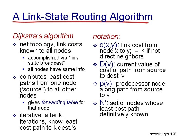
A Link-State Routing Algorithm Dijkstra’s algorithm v net topology, link costs known to all nodes § accomplished via “link state broadcast” § all nodes have same info v computes least cost paths from one node (‘source”) to all other nodes § gives forwarding table for that node v iterative: after k iterations, know least cost path to k dest. ’s notation: v c(x, y): link cost from v v v node x to y; = ∞ if not direct neighbors D(v): current value of cost of path from source to dest. v p(v): predecessor node along path from source to v N': set of nodes whose least cost path definitively known Network Layer 4 -38

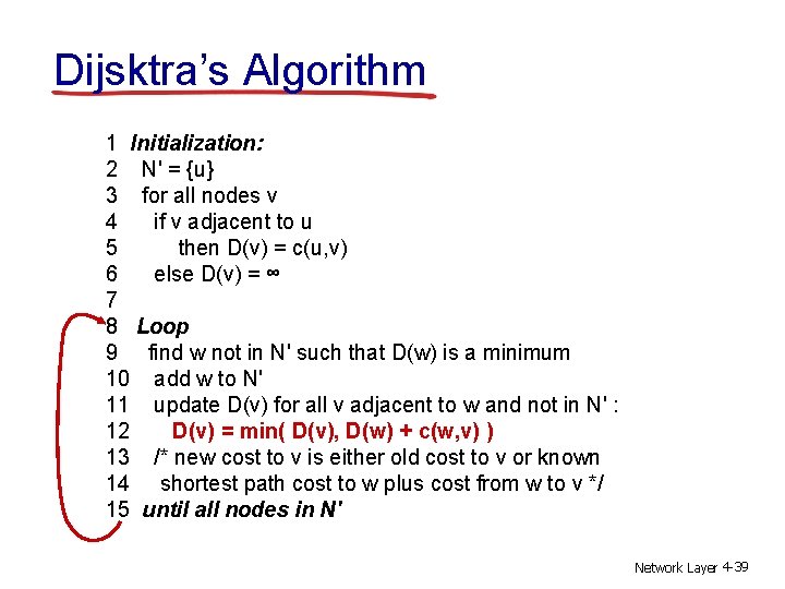
Dijsktra’s Algorithm 1 Initialization: 2 N' = {u} 3 for all nodes v 4 if v adjacent to u 5 then D(v) = c(u, v) 6 else D(v) = ∞ 7 8 Loop 9 find w not in N' such that D(w) is a minimum 10 add w to N' 11 update D(v) for all v adjacent to w and not in N' : 12 D(v) = min( D(v), D(w) + c(w, v) ) 13 /* new cost to v is either old cost to v or known 14 shortest path cost to w plus cost from w to v */ 15 until all nodes in N' Network Layer 4 -39

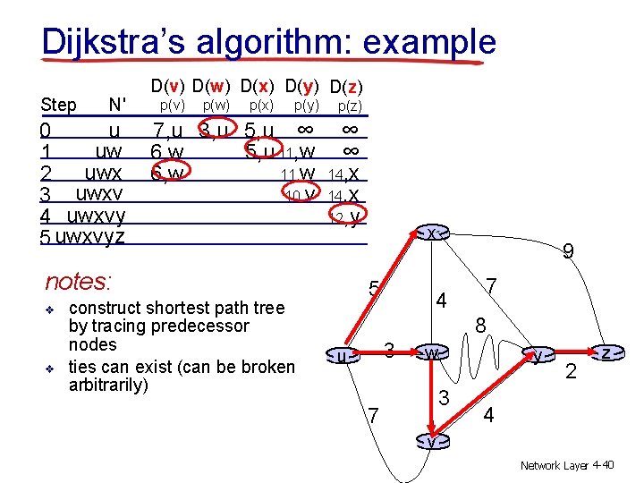
Dijkstra’s algorithm: example Step N' u 0 uw 1 uwx 2 3 uwxv 4 uwxvy 5 uwxvyz D(v) D(w) D(x) D(y) D(z) p(v) p(w) p(x) p(y) 7, u 3, u 5, u ∞ 5, u 11, w 6, w 10, v p(z) ∞ ∞ 14, x 12, y notes: v v construct shortest path tree by tracing predecessor nodes ties can exist (can be broken arbitrarily) x 5 9 4 7 8 3 u w y 3 7 2 z 4 v Network Layer 4 -40

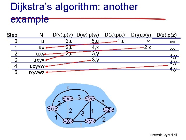
Dijkstra’s algorithm: another example Step 0 1 2 3 4 5 N' u ux uxyvwz D(v), p(v) D(w), p(w) 2, u 5, u 2, u 4, x 2, u 3, y D(x), p(x) 1, u D(y), p(y) ∞ 2, x D(z), p(z) ∞ ∞ 4, y 5 u 2 1 v 2 x 3 w 3 1 1 y 5 z 2 Network Layer 4 -41

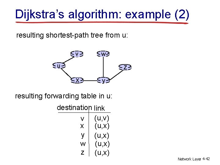
Dijkstra’s algorithm: example (2) resulting shortest-path tree from u: v w u z x y resulting forwarding table in u: destination link v (u, v) x (u, x) y (u, x) w (u, x) z (u, x) Network Layer 4 -42

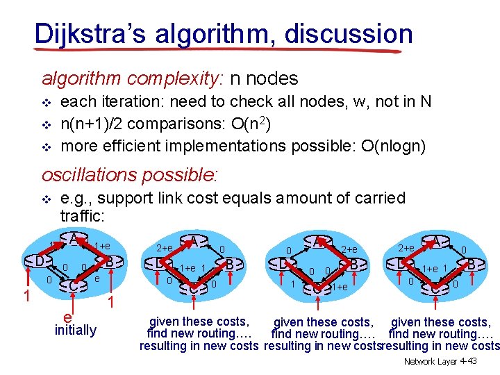
Dijkstra’s algorithm, discussion algorithm complexity: n nodes v v v each iteration: need to check all nodes, w, not in N n(n+1)/2 comparisons: O(n 2) more efficient implementations possible: O(nlogn) oscillations possible: v e. g. , support link cost equals amount of carried traffic: A 1 D 1 B 0 0 0 1+e C e e initially 2+e D 0 C 0 B 1+e 1 0 1 A 0 D A 0 1 C 2+e B 0 1+e 2+e D A 0 B 1+e 1 0 C 0 given these costs, find new routing…. resulting in new costsresulting in new costs Network Layer 4 -43

The End is Near!