Lecture 7 Inductive Inference MDL and PAC Learning

Lecture 7: Inductive Inference MDL and PAC Learning

Oxford English Dictionary l Induction is ``the process of inferring a general law or principle from the observations of particular instances''. l Science is induction: from observed data to physical laws. l But, how? …

Epicurus: Multiple Explanations l Greek philosopher of science Epicurus (342 -270 BC) proposed the Principle of Multiple Explanations: If more than one theory is consistent with the observations, keep all theories. l ``There also some things for which it is not enough to state a single cause, but several, of which one, however, is the case. Just as if you were to see the lifeless corpse of a man lying far away, it would be fitting to state all the causes of death in order that the single cause of this death may be stated. For you would not be able to establish conclusively that he died by the sword or of cold or of illness or perhaps by poison, but we know that there is something of this kind that happened to him. '‘ [Lucretius]

Occam’s Razor Commonly attributed to William of Ockham (1290 --1349). This was formulated about fifteen hundred years after Epicurus. In sharp contrast to the principle of multiple explanations, it states: Entities should not be multiplied beyond necessity. l Commonly explained as: when have choices, choose the simplest theory. l Bertrand Russell: ``It is vain to do with more what can be done with fewer. '‘ l Newton (Principia): ``Natura enim simplex est, et rerum causis superfluis non luxuriat''. l

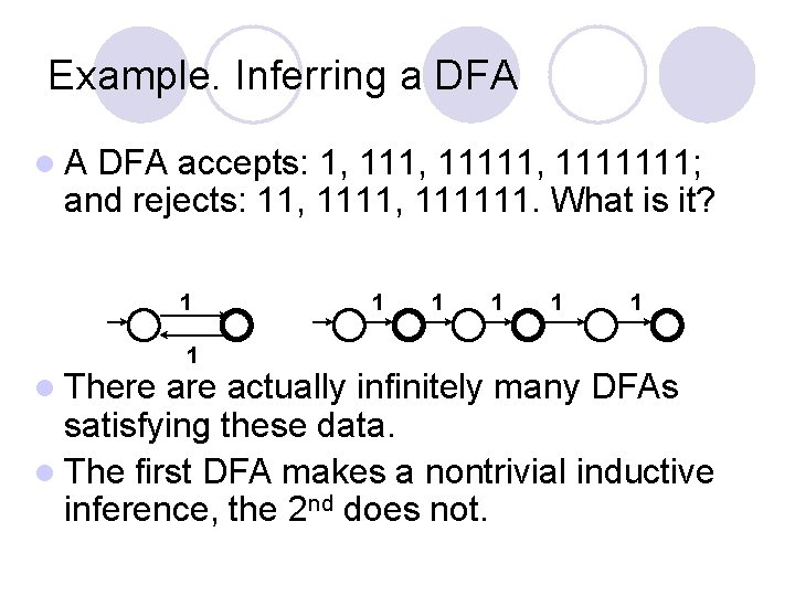
Example. Inferring a DFA l. A DFA accepts: 1, 11111, 1111111; and rejects: 11, 111111. What is it? 1 l There 1 1 1 are actually infinitely many DFAs satisfying these data. l The first DFA makes a nontrivial inductive inference, the 2 nd does not.

Exampe. History of Science Maxwell's (1831 -1879)'s equations say that: (a) An oscillating magnetic field gives rise to an oscillating electric field; (b) an oscillating electric field gives rise to an oscillating magnetic field. Item (a) was known from M. Faraday's experiments. However (b) is a theoretical inference by Maxwell and his aesthetic appreciation of simplicity. The existence of such electromagnetic waves was demonstrated by the experiments of H. Hertz in 1888, 8 years after Maxwell's death, and this opened the new field of radio communication. Maxwell's theory is even relativistically invariant. This was long before Einstein’s special relativity. As a matter of fact, it is even likely that Maxwell's theory influenced Einstein’s 1905 paper on relativity which was actually titled `On the electrodynamics of moving bodies'. l J. Kemeny, a former assistant to Einstein, explains the transition from the special theory to the general theory of relativity: At the time, there were no new facts that failed to be explained by the special theory of relativity. Einstein was purely motivated by his conviction that the special theory was not the simplest theory which can explain all the observed facts. Reducing the number of variables obviously simplifies a theory. By the requirement of general covariance Einstein succeeded in replacing the previous ‘gravitational mass' and `inertial mass' by a single concept. l Double helix vs triple helix --- 1953, Watson & Crick l

Counter Example. l Once upon a time, there was a little girl named Emma had never eaten a banana, nor had she ever been on a train. One day she had to journey from New York to Pittsburgh by train. To relieve Emma's anxiety, her mother gave her a large bag of bananas. At Emma's first bite of her banana, the train plunged into a tunnel. At the second bite, the train broke into daylight again. At the third bite, Lo! into a tunnel; the fourth bite, La! into daylight again. And so on all the way to Pittsburgh. Emma, being a bright little girl, told her grandpa at the station: ``Every odd bite of a banana makes you blind; every even bite puts things right again. '‘ (N. R. Hanson, Perception & Discovery)

What is “simplicity”? l We still have not defined `simplicity'. How does one define it? Is ¼ simpler than 1/10? Is 1/3 simpler than 2/3? Note that saying that there are 1/3 white balls in the urn is the same as that of 2/3 black balls. If one wants to infer polynomials, is x 100 +1 more complicated than 13 x 17 + 5 x 3 + 7 x +11? l Can a thing be simple under one definition of simplicity and not simple under another?

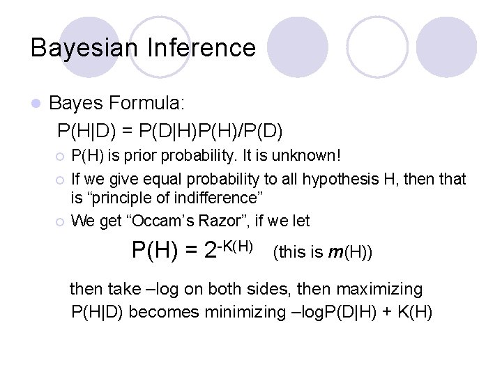
Bayesian Inference l Bayes Formula: P(H|D) = P(D|H)P(H)/P(D) ¡ ¡ ¡ P(H) is prior probability. It is unknown! If we give equal probability to all hypothesis H, then that is “principle of indifference” We get “Occam’s Razor”, if we let P(H) = 2 -K(H) (this is m(H)) then take –log on both sides, then maximizing P(H|D) becomes minimizing –log. P(D|H) + K(H)

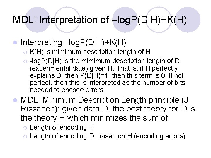
MDL: Interpretation of –log. P(D|H)+K(H) l Interpreting –log. P(D|H)+K(H) ¡ ¡ l K(H) is mimimum description length of H -log. P(D|H) is the mimimum description length of D (experimental data) given H. That is, if H perfectly explains D, then P(D|H)=1, then this term is 0. If not perfect, then this is interpreted as the number of bits needed to encode errors. MDL: Minimum Description Length principle (J. Rissanen): given data D, the best theory for D is theory H which minimizes the sum of ¡ ¡ Length of encoding H Length of encoding D, based on H (encoding errors)

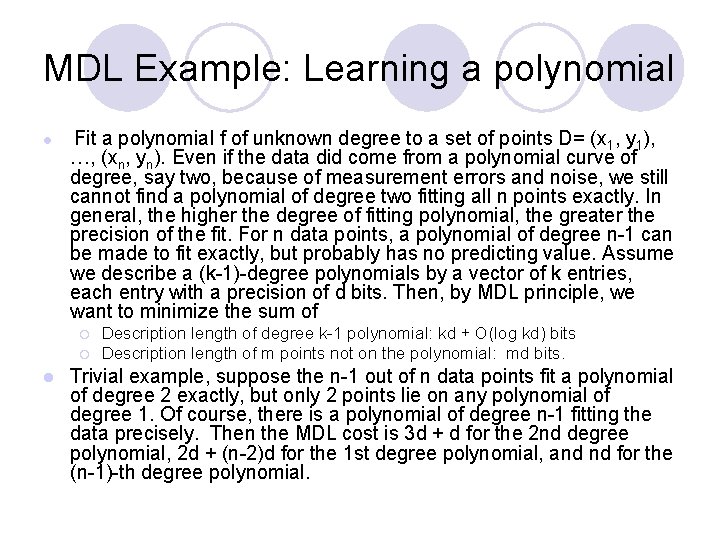
MDL Example: Learning a polynomial l Fit a polynomial f of unknown degree to a set of points D= (x 1, y 1), …, (xn, yn). Even if the data did come from a polynomial curve of degree, say two, because of measurement errors and noise, we still cannot find a polynomial of degree two fitting all n points exactly. In general, the higher the degree of fitting polynomial, the greater the precision of the fit. For n data points, a polynomial of degree n-1 can be made to fit exactly, but probably has no predicting value. Assume we describe a (k-1)-degree polynomials by a vector of k entries, each entry with a precision of d bits. Then, by MDL principle, we want to minimize the sum of ¡ ¡ l Description length of degree k-1 polynomial: kd + O(log kd) bits Description length of m points not on the polynomial: md bits. Trivial example, suppose the n-1 out of n data points fit a polynomial of degree 2 exactly, but only 2 points lie on any polynomial of degree 1. Of course, there is a polynomial of degree n-1 fitting the data precisely. Then the MDL cost is 3 d + d for the 2 nd degree polynomial, 2 d + (n-2)d for the 1 st degree polynomial, and nd for the (n-1)-th degree polynomial.

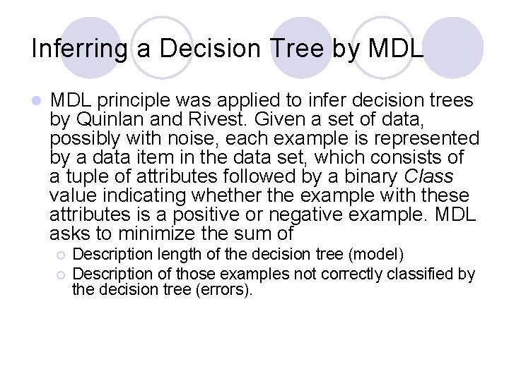
Inferring a Decision Tree by MDL l MDL principle was applied to infer decision trees by Quinlan and Rivest. Given a set of data, possibly with noise, each example is represented by a data item in the data set, which consists of a tuple of attributes followed by a binary Class value indicating whether the example with these attributes is a positive or negative example. MDL asks to minimize the sum of ¡ ¡ Description length of the decision tree (model) Description of those examples not correctly classified by the decision tree (errors).

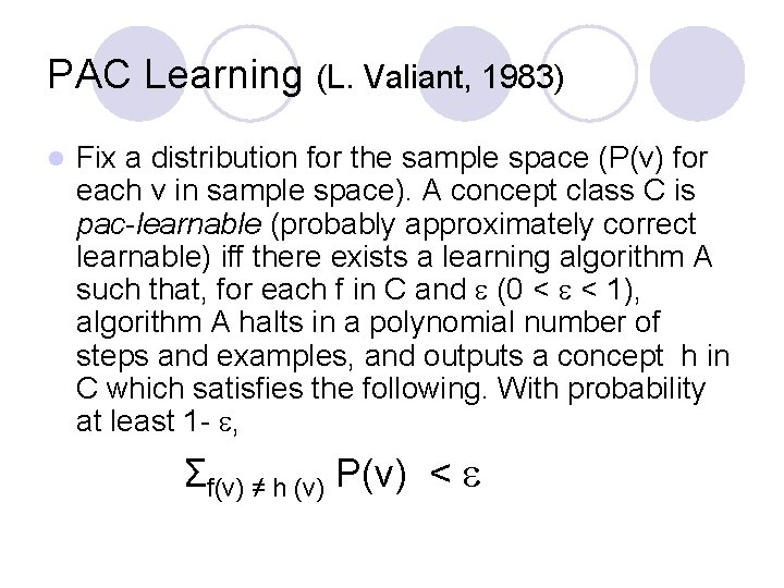
PAC Learning (L. Valiant, 1983) l Fix a distribution for the sample space (P(v) for each v in sample space). A concept class C is pac-learnable (probably approximately correct learnable) iff there exists a learning algorithm A such that, for each f in C and (0 < < 1), algorithm A halts in a polynomial number of steps and examples, and outputs a concept h in C which satisfies the following. With probability at least 1 - , Σf(v) ≠ h (v) P(v) <

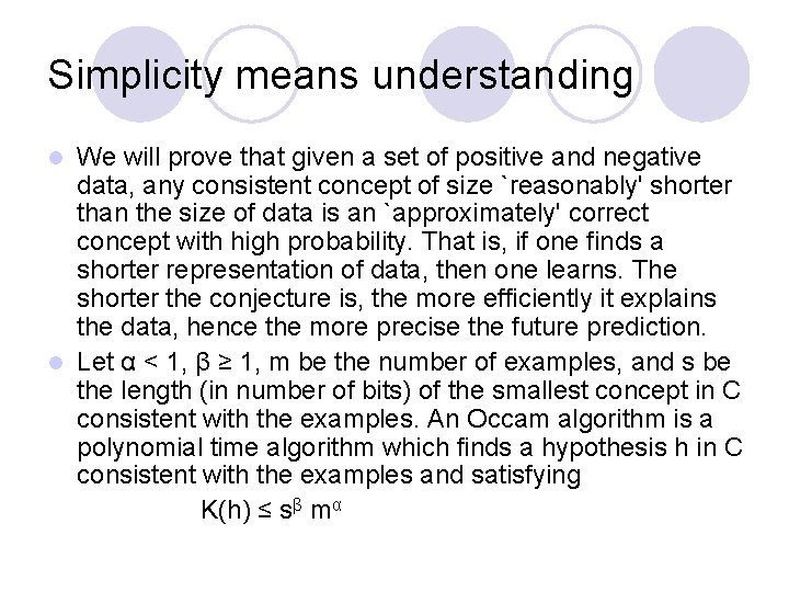
Simplicity means understanding We will prove that given a set of positive and negative data, any consistent concept of size `reasonably' shorter than the size of data is an `approximately' correct concept with high probability. That is, if one finds a shorter representation of data, then one learns. The shorter the conjecture is, the more efficiently it explains the data, hence the more precise the future prediction. l Let α < 1, β ≥ 1, m be the number of examples, and s be the length (in number of bits) of the smallest concept in C consistent with the examples. An Occam algorithm is a polynomial time algorithm which finds a hypothesis h in C consistent with the examples and satisfying K(h) ≤ sβ mα l

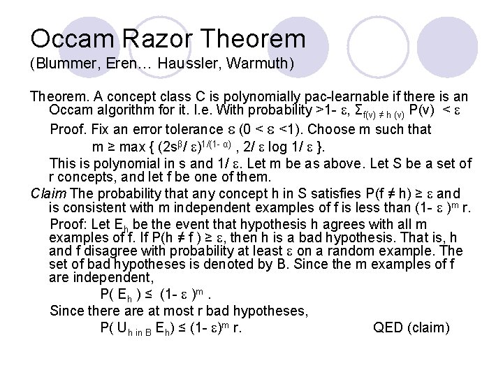
Occam Razor Theorem (Blummer, Eren… Haussler, Warmuth) Theorem. A concept class C is polynomially pac-learnable if there is an Occam algorithm for it. I. e. With probability >1 - , Σf(v) ≠ h (v) P(v) < Proof. Fix an error tolerance (0 < <1). Choose m such that m ≥ max { (2 sβ/ )1/(1 - α) , 2/ log 1/ }. This is polynomial in s and 1/ . Let m be as above. Let S be a set of r concepts, and let f be one of them. Claim The probability that any concept h in S satisfies P(f ≠ h) ≥ and is consistent with m independent examples of f is less than (1 - )m r. Proof: Let Eh be the event that hypothesis h agrees with all m examples of f. If P(h ≠ f ) ≥ , then h is a bad hypothesis. That is, h and f disagree with probability at least on a random example. The set of bad hypotheses is denoted by B. Since the m examples of f are independent, P( Eh ) ≤ (1 - )m. Since there at most r bad hypotheses, P( Uh in B Eh) ≤ (1 - )m r. QED (claim)

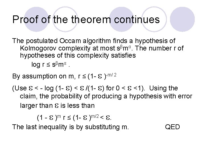
Proof of theorem continues The postulated Occam algorithm finds a hypothesis of Kolmogorov complexity at most sβmα. The number r of hypotheses of this complexity satisfies log r ≤ sβmα. By assumption on m, r ≤ (1 - )-m/ 2 (Use < - log (1 - ) < /(1 - ) for 0 < <1). Using the claim, the probability of producing a hypothesis with error larger than is less than (1 - )m r ≤ (1 - )m/2 < . The last inequality is by substituting m. QED

Summary l The simpler, the better.