Lecture 12 Parametric Signal Modeling XILIANG LUO 201411

Lecture 12: Parametric Signal Modeling XILIANG LUO 2014/11 1

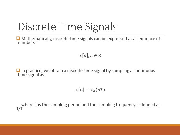
Discrete Time Signals

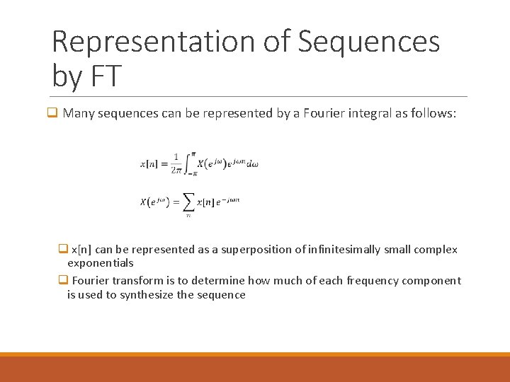
Representation of Sequences by FT q Many sequences can be represented by a Fourier integral as follows: q x[n] can be represented as a superposition of infinitesimally small complex exponentials q Fourier transform is to determine how much of each frequency component is used to synthesize the sequence

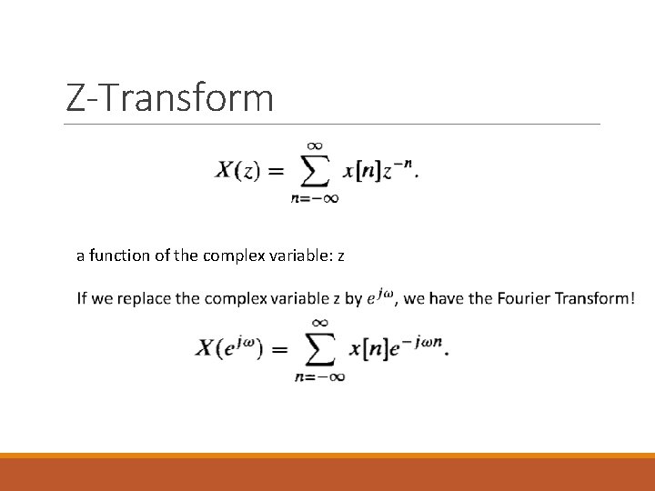
Z-Transform a function of the complex variable: z

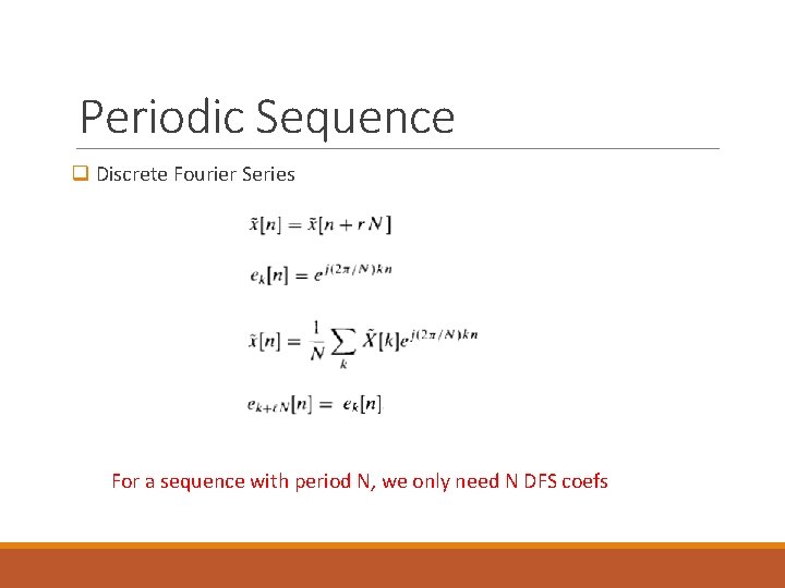
Periodic Sequence q Discrete Fourier Series For a sequence with period N, we only need N DFS coefs

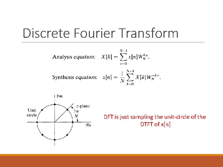
Discrete Fourier Transform DFT is just sampling the unit-circle of the DTFT of x[n]

Parametric Signal Modeling A signal is represented by a mathematical model which has a Predefined structure involving a limited number of parameters. A given signal is represented by choosing the specific set of parameters that results in the model output being as close as possible in some prescribed sense to the given signal. 7

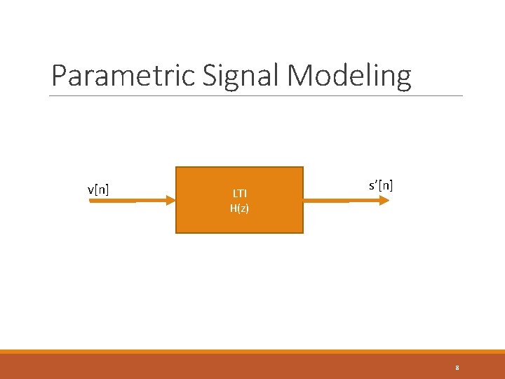
Parametric Signal Modeling v[n] LTI H(z) s’[n] 8

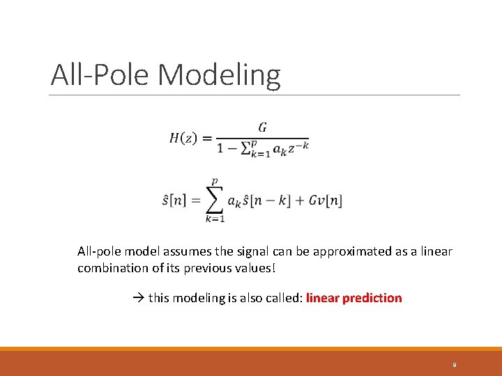
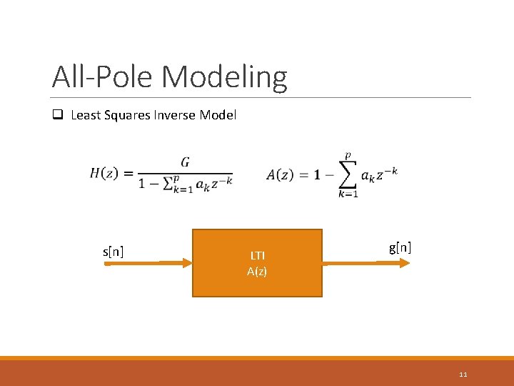
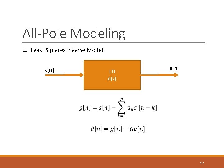
All-Pole Modeling All-pole model assumes the signal can be approximated as a linear combination of its previous values! this modeling is also called: linear prediction 9

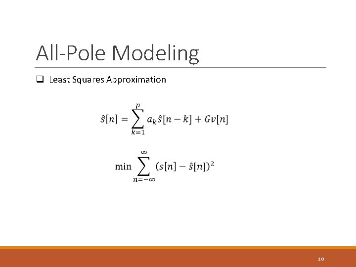
All-Pole Modeling q Least Squares Approximation 10

All-Pole Modeling q Least Squares Inverse Model s[n] LTI A(z) g[n] 11

All-Pole Modeling q Least Squares Inverse Model s[n] LTI A(z) g[n] 12

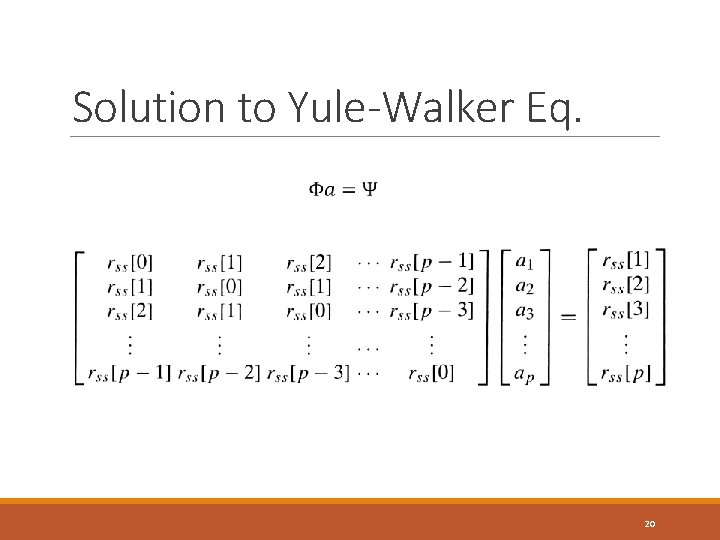
All-Pole Modeling q Least Squares Inverse Model Yule-Walker equations 13

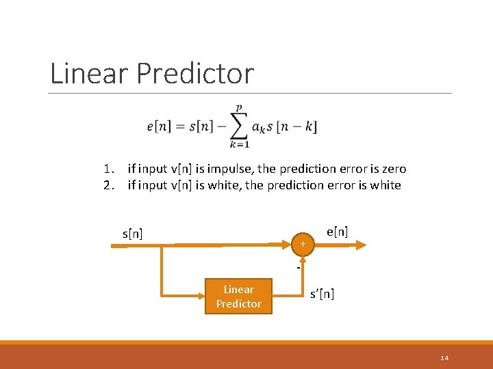
Linear Predictor 1. if input v[n] is impulse, the prediction error is zero 2. if input v[n] is white, the prediction error is white s[n] e[n] + Linear Predictor s’[n] 14

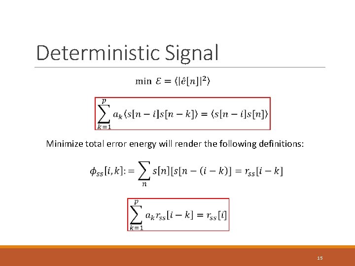
Deterministic Signal Minimize total error energy will render the following definitions: 15

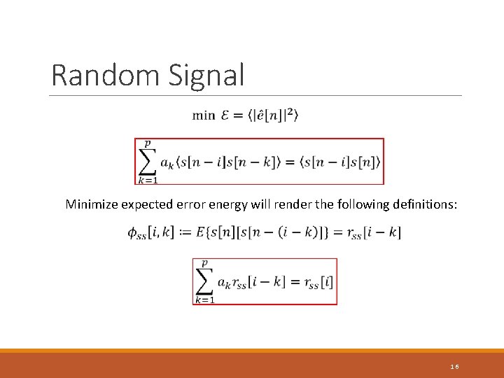
Random Signal Minimize expected error energy will render the following definitions: 16

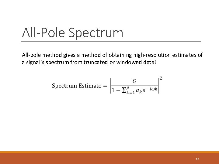
All-Pole Spectrum All-pole method gives a method of obtaining high-resolution estimates of a signal’s spectrum from truncated or windowed data! 17

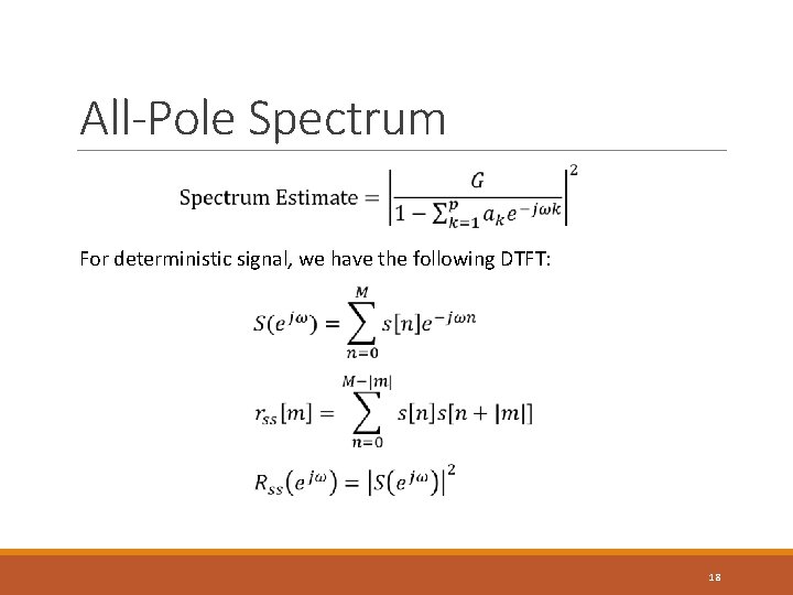
All-Pole Spectrum For deterministic signal, we have the following DTFT: 18

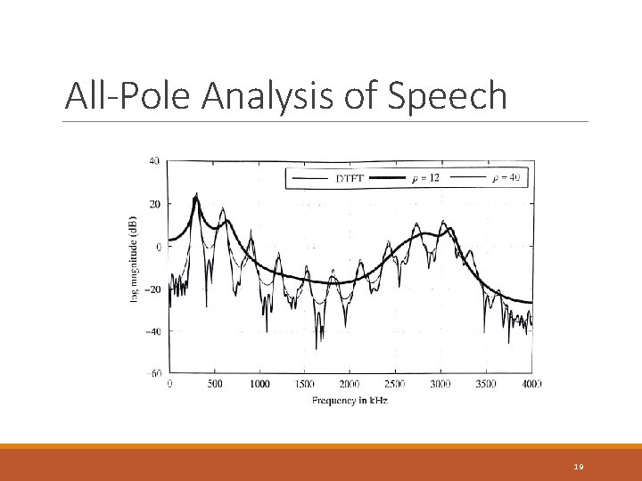
All-Pole Analysis of Speech 19

Solution to Yule-Walker Eq. 20

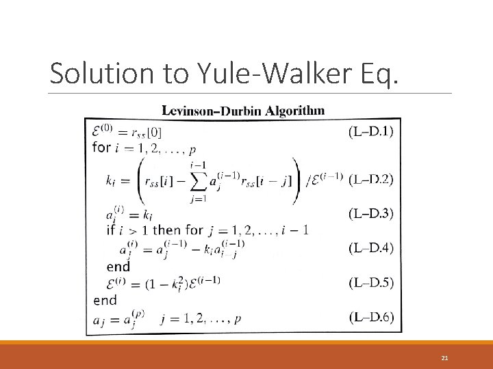
Solution to Yule-Walker Eq. 21

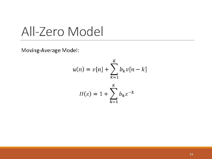
All-Zero Model Moving-Average Model: 22

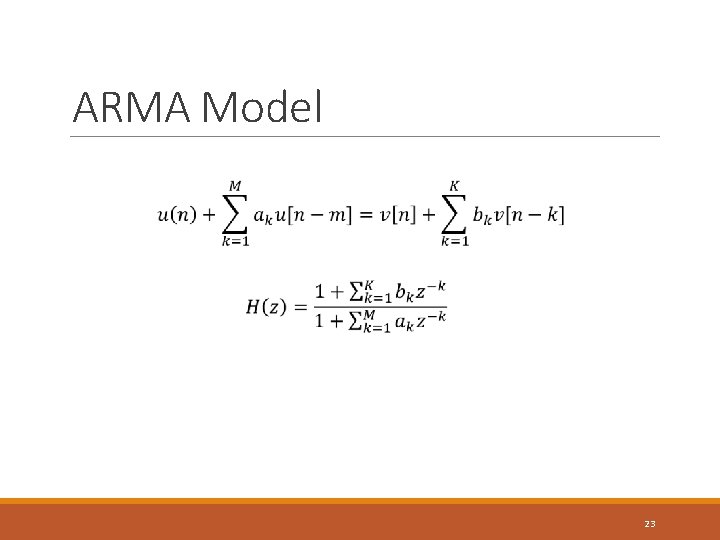
ARMA Model 23

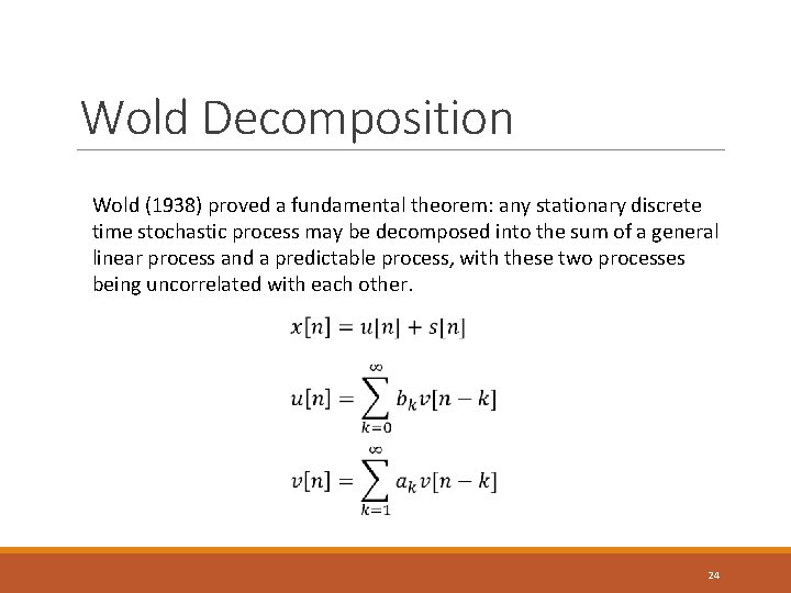
Wold Decomposition Wold (1938) proved a fundamental theorem: any stationary discrete time stochastic process may be decomposed into the sum of a general linear process and a predictable process, with these two processes being uncorrelated with each other. 24