Learning for Text Categorization 1 Text Categorization Representations

Learning for Text Categorization 1

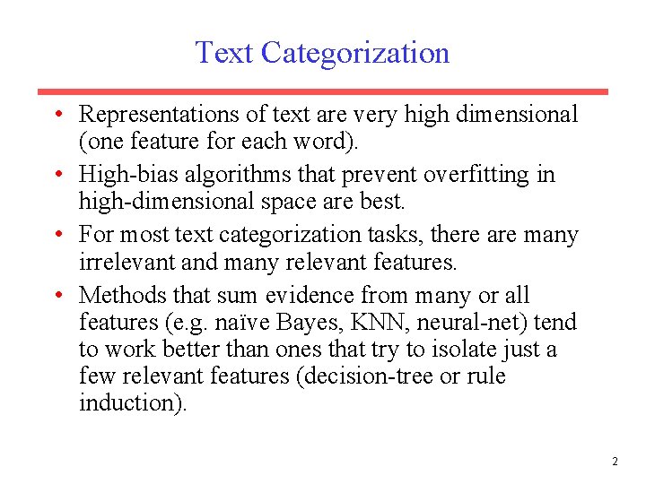
Text Categorization • Representations of text are very high dimensional (one feature for each word). • High-bias algorithms that prevent overfitting in high-dimensional space are best. • For most text categorization tasks, there are many irrelevant and many relevant features. • Methods that sum evidence from many or all features (e. g. naïve Bayes, KNN, neural-net) tend to work better than ones that try to isolate just a few relevant features (decision-tree or rule induction). 2

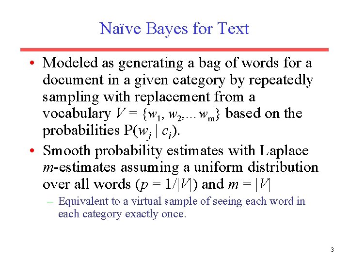
Naïve Bayes for Text • Modeled as generating a bag of words for a document in a given category by repeatedly sampling with replacement from a vocabulary V = {w 1, w 2, …wm} based on the probabilities P(wj | ci). • Smooth probability estimates with Laplace m-estimates assuming a uniform distribution over all words (p = 1/|V|) and m = |V| – Equivalent to a virtual sample of seeing each word in each category exactly once. 3

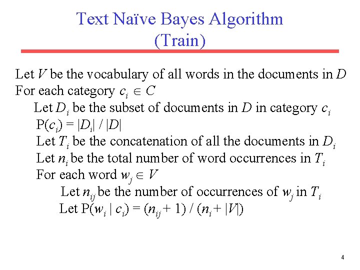
Text Naïve Bayes Algorithm (Train) Let V be the vocabulary of all words in the documents in D For each category ci C Let Di be the subset of documents in D in category ci P(ci) = |Di| / |D| Let Ti be the concatenation of all the documents in Di Let ni be the total number of word occurrences in Ti For each word wj V Let nij be the number of occurrences of wj in Ti Let P(wi | ci) = (nij + 1) / (ni + |V|) 4

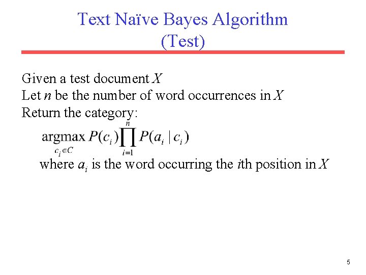
Text Naïve Bayes Algorithm (Test) Given a test document X Let n be the number of word occurrences in X Return the category: where ai is the word occurring the ith position in X 5

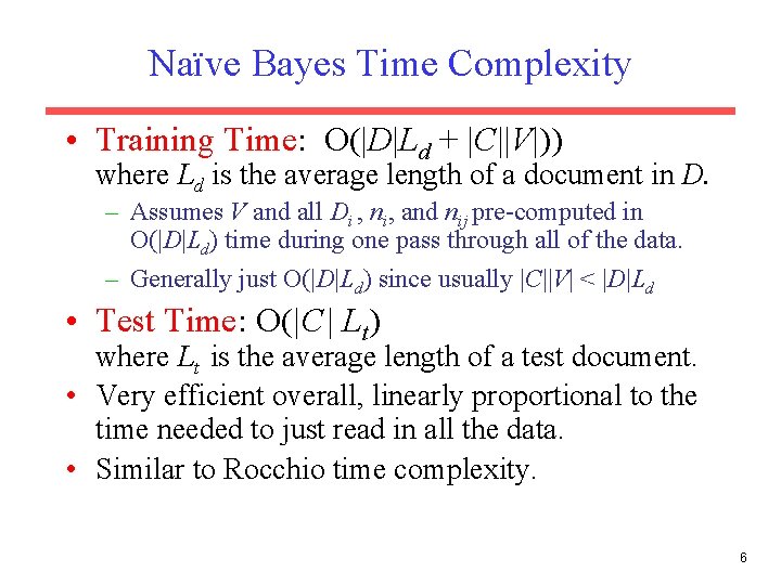
Naïve Bayes Time Complexity • Training Time: O(|D|Ld + |C||V|)) where Ld is the average length of a document in D. – Assumes V and all Di , ni, and nij pre-computed in O(|D|Ld) time during one pass through all of the data. – Generally just O(|D|Ld) since usually |C||V| < |D|Ld • Test Time: O(|C| Lt) where Lt is the average length of a test document. • Very efficient overall, linearly proportional to the time needed to just read in all the data. • Similar to Rocchio time complexity. 6

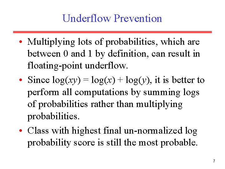
Underflow Prevention • Multiplying lots of probabilities, which are between 0 and 1 by definition, can result in floating-point underflow. • Since log(xy) = log(x) + log(y), it is better to perform all computations by summing logs of probabilities rather than multiplying probabilities. • Class with highest final un-normalized log probability score is still the most probable. 7

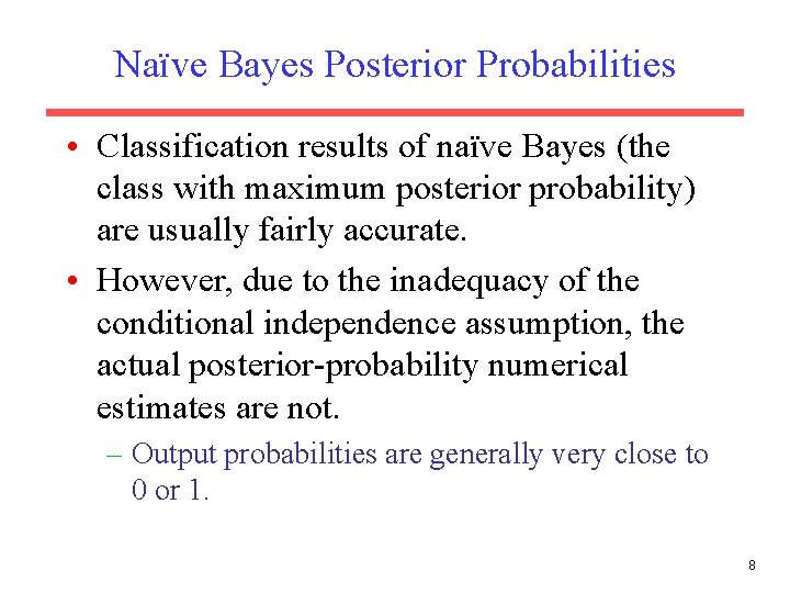
Naïve Bayes Posterior Probabilities • Classification results of naïve Bayes (the class with maximum posterior probability) are usually fairly accurate. • However, due to the inadequacy of the conditional independence assumption, the actual posterior-probability numerical estimates are not. – Output probabilities are generally very close to 0 or 1. 8

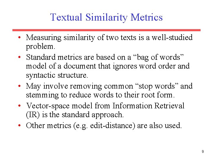
Textual Similarity Metrics • Measuring similarity of two texts is a well-studied problem. • Standard metrics are based on a “bag of words” model of a document that ignores word order and syntactic structure. • May involve removing common “stop words” and stemming to reduce words to their root form. • Vector-space model from Information Retrieval (IR) is the standard approach. • Other metrics (e. g. edit-distance) are also used. 9

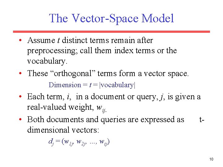
The Vector-Space Model • Assume t distinct terms remain after preprocessing; call them index terms or the vocabulary. • These “orthogonal” terms form a vector space. Dimension = t = |vocabulary| • Each term, i, in a document or query, j, is given a real-valued weight, wij. • Both documents and queries are expressed as tdimensional vectors: dj = (w 1 j, w 2 j, …, wtj) 10

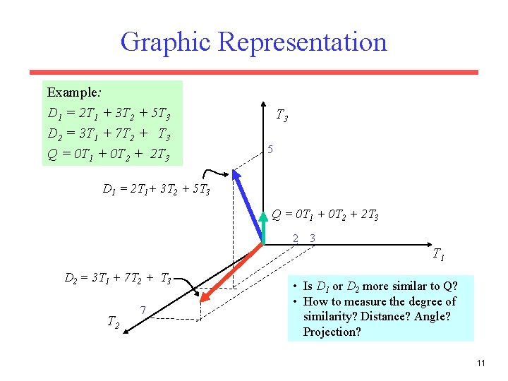
Graphic Representation Example: D 1 = 2 T 1 + 3 T 2 + 5 T 3 D 2 = 3 T 1 + 7 T 2 + T 3 Q = 0 T 1 + 0 T 2 + 2 T 3 5 D 1 = 2 T 1+ 3 T 2 + 5 T 3 Q = 0 T 1 + 0 T 2 + 2 T 3 2 3 T 1 D 2 = 3 T 1 + 7 T 2 + T 3 T 2 7 • Is D 1 or D 2 more similar to Q? • How to measure the degree of similarity? Distance? Angle? Projection? 11

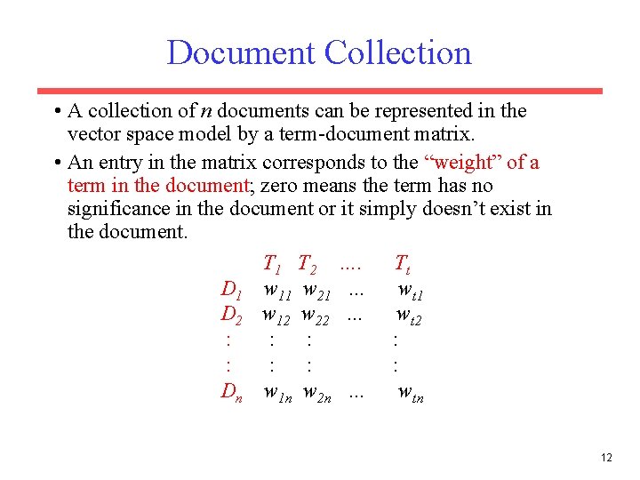
Document Collection • A collection of n documents can be represented in the vector space model by a term-document matrix. • An entry in the matrix corresponds to the “weight” of a term in the document; zero means the term has no significance in the document or it simply doesn’t exist in the document. T 1 T 2 …. Tt D 1 w 11 w 21 … wt 1 D 2 w 12 w 22 … wt 2 : : : : Dn w 1 n w 2 n … wtn 12

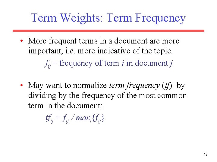
Term Weights: Term Frequency • More frequent terms in a document are more important, i. e. more indicative of the topic. fij = frequency of term i in document j • May want to normalize term frequency (tf) by dividing by the frequency of the most common term in the document: tfij = fij / maxi{fij} 13

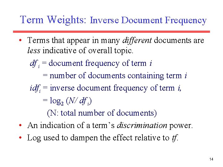
Term Weights: Inverse Document Frequency • Terms that appear in many different documents are less indicative of overall topic. df i = document frequency of term i = number of documents containing term i idfi = inverse document frequency of term i, = log 2 (N/ df i) (N: total number of documents) • An indication of a term’s discrimination power. • Log used to dampen the effect relative to tf. 14

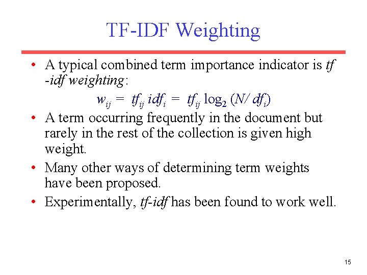
TF-IDF Weighting • A typical combined term importance indicator is tf -idf weighting: wij = tfij idfi = tfij log 2 (N/ dfi) • A term occurring frequently in the document but rarely in the rest of the collection is given high weight. • Many other ways of determining term weights have been proposed. • Experimentally, tf-idf has been found to work well. 15

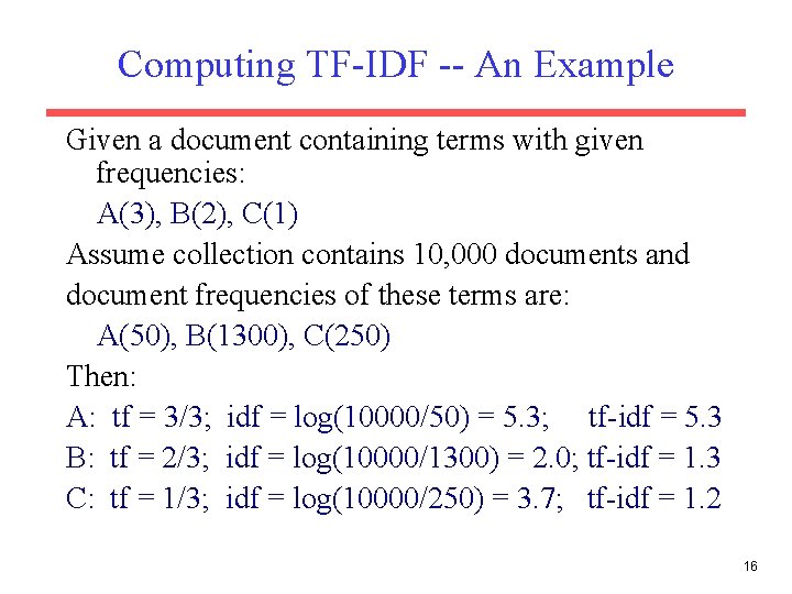
Computing TF-IDF -- An Example Given a document containing terms with given frequencies: A(3), B(2), C(1) Assume collection contains 10, 000 documents and document frequencies of these terms are: A(50), B(1300), C(250) Then: A: tf = 3/3; idf = log(10000/50) = 5. 3; tf-idf = 5. 3 B: tf = 2/3; idf = log(10000/1300) = 2. 0; tf-idf = 1. 3 C: tf = 1/3; idf = log(10000/250) = 3. 7; tf-idf = 1. 2 16

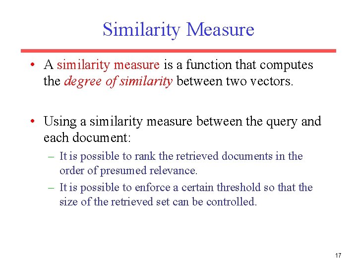
Similarity Measure • A similarity measure is a function that computes the degree of similarity between two vectors. • Using a similarity measure between the query and each document: – It is possible to rank the retrieved documents in the order of presumed relevance. – It is possible to enforce a certain threshold so that the size of the retrieved set can be controlled. 17

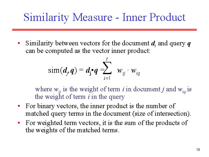
Similarity Measure - Inner Product • Similarity between vectors for the document di and query q can be computed as the vector inner product: sim(dj, q) = dj • q = wij · wiq where wij is the weight of term i in document j and wiq is the weight of term i in the query • For binary vectors, the inner product is the number of matched query terms in the document (size of intersection). • For weighted term vectors, it is the sum of the products of the weights of the matched terms. 18

Properties of Inner Product • The inner product is unbounded. • Favors long documents with a large number of unique terms. • Measures how many terms matched but not how many terms are not matched. 19

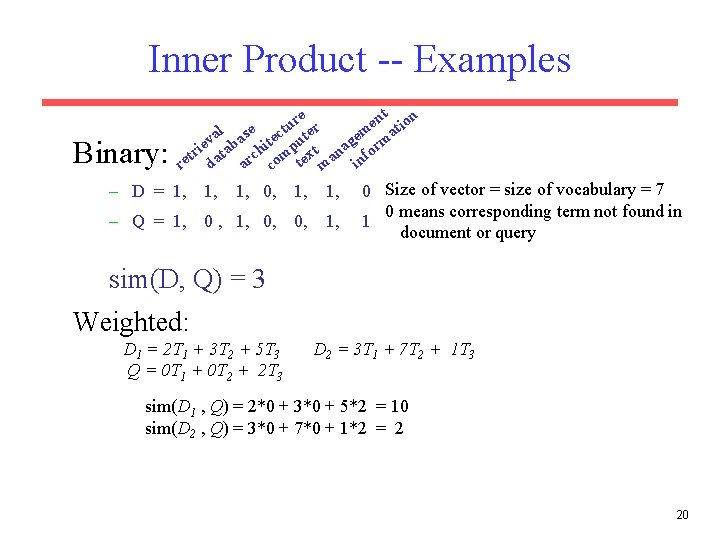
Inner Product -- Examples Binary: nt ion re r e u m at al ase tect ute e v g e ab hi p t a form i r n t c t m x re da ar co te ma in – D = 1, 1, 1, 0, 1, 1, – Q = 1, 0 , 1, 0, 0, 1, 0 Size of vector = size of vocabulary = 7 0 means corresponding term not found in 1 document or query sim(D, Q) = 3 Weighted: D 1 = 2 T 1 + 3 T 2 + 5 T 3 Q = 0 T 1 + 0 T 2 + 2 T 3 D 2 = 3 T 1 + 7 T 2 + 1 T 3 sim(D 1 , Q) = 2*0 + 3*0 + 5*2 = 10 sim(D 2 , Q) = 3*0 + 7*0 + 1*2 = 2 20

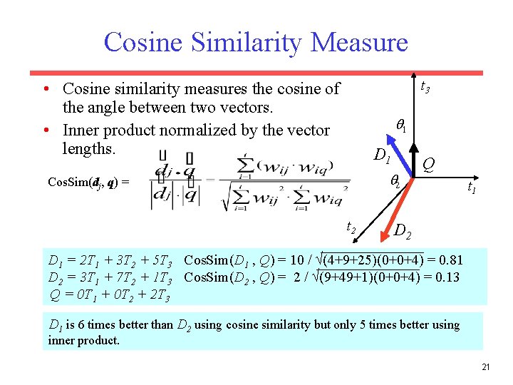
Cosine Similarity Measure t 3 • Cosine similarity measures the cosine of the angle between two vectors. • Inner product normalized by the vector lengths. 1 D 1 2 Cos. Sim(dj, q) = t 2 Q t 1 D 2 D 1 = 2 T 1 + 3 T 2 + 5 T 3 Cos. Sim(D 1 , Q) = 10 / (4+9+25)(0+0+4) = 0. 81 D 2 = 3 T 1 + 7 T 2 + 1 T 3 Cos. Sim(D 2 , Q) = 2 / (9+49+1)(0+0+4) = 0. 13 Q = 0 T 1 + 0 T 2 + 2 T 3 D 1 is 6 times better than D 2 using cosine similarity but only 5 times better using inner product. 21

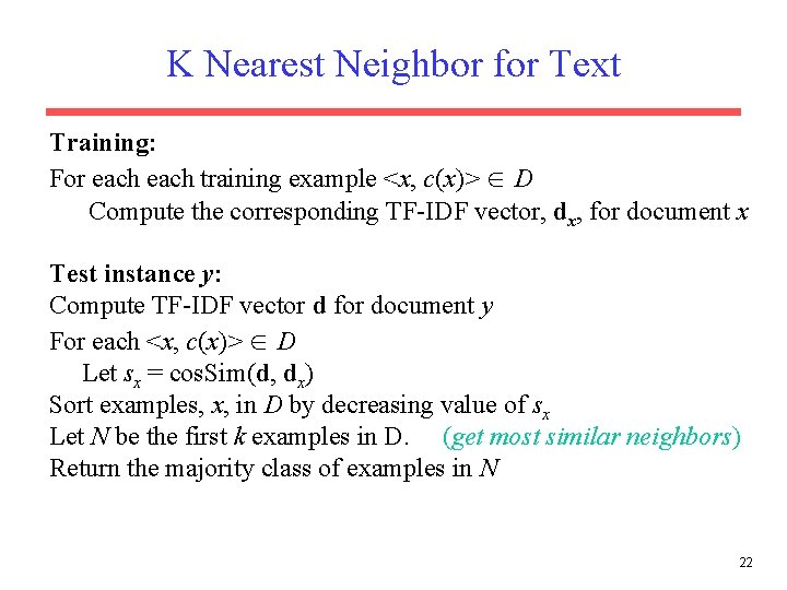
K Nearest Neighbor for Text Training: For each training example <x, c(x)> D Compute the corresponding TF-IDF vector, dx, for document x Test instance y: Compute TF-IDF vector d for document y For each <x, c(x)> D Let sx = cos. Sim(d, dx) Sort examples, x, in D by decreasing value of sx Let N be the first k examples in D. (get most similar neighbors) Return the majority class of examples in N 22

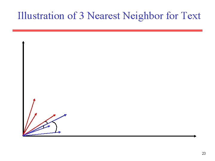
Illustration of 3 Nearest Neighbor for Text 23

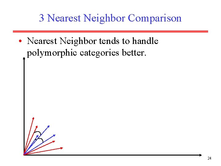
3 Nearest Neighbor Comparison • Nearest Neighbor tends to handle polymorphic categories better. 24

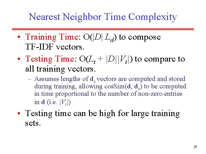
Nearest Neighbor Time Complexity • Training Time: O(|D| Ld) to compose TF-IDF vectors. • Testing Time: O(Lt + |D||Vt|) to compare to all training vectors. – Assumes lengths of dx vectors are computed and stored during training, allowing cos. Sim(d, dx) to be computed in time proportional to the number of non-zero entries in d (i. e. |Vt|) • Testing time can be high for large training sets. 25

Nearest Neighbor with Inverted Index • Determining k nearest neighbors is the same as determining the k best retrievals using the test document as a query to a database of training documents. • Use standard VSR inverted index methods to find the k nearest neighbors. • Testing Time: O(B|Vt|) where B is the average number of training documents in which a test-document word appears. • Therefore, overall classification is O(Lt + B|Vt|) – Typically B << |D| 26

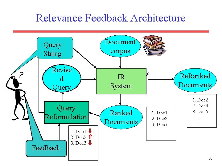
Relevance Feedback in IR • After initial retrieval results are presented, allow the user to provide feedback on the relevance of one or more of the retrieved documents. • Use this feedback information to reformulate the query. • Produce new results based on reformulated query. • Allows more interactive, multi-pass process. 27

Relevance Feedback Architecture Document corpus Query String Revise d Query Reformulation Feedback 1. Doc 1 2. Doc 2 3. Doc 3 . . Rankings Re. Ranked Documents IR System Ranked Documents 1. Doc 1 2. Doc 2 3. Doc 3. . 1. Doc 2 2. Doc 4 3. Doc 5. . 28

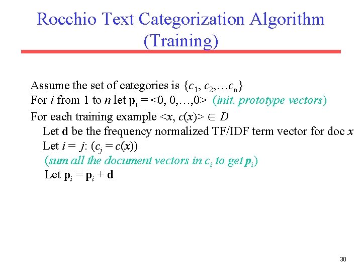
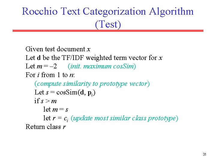
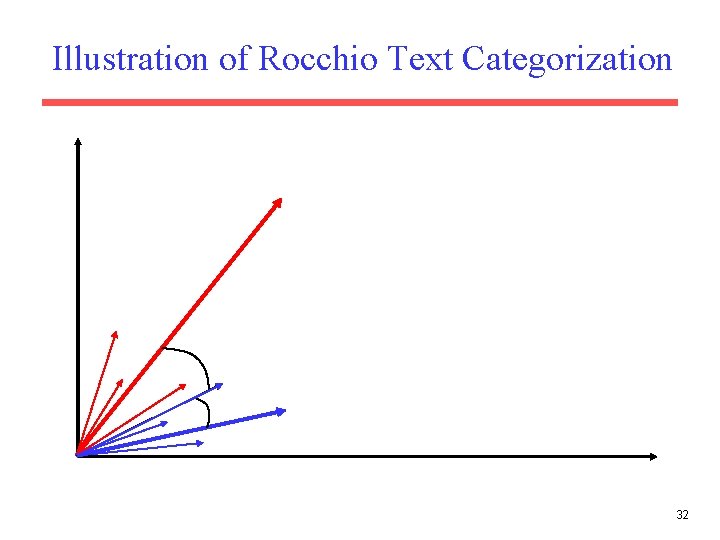
Using Relevance Feedback (Rocchio) • Relevance feedback methods can be adapted for text categorization. • Use standard TF/IDF weighted vectors to represent text documents (normalized by maximum term frequency). • For each category, compute a prototype vector by summing the vectors of the training documents in the category. • Assign test documents to the category with the closest prototype vector based on cosine similarity. 29

Rocchio Text Categorization Algorithm (Training) Assume the set of categories is {c 1, c 2, …cn} For i from 1 to n let pi = <0, 0, …, 0> (init. prototype vectors) For each training example <x, c(x)> D Let d be the frequency normalized TF/IDF term vector for doc x Let i = j: (cj = c(x)) (sum all the document vectors in ci to get pi) Let pi = pi + d 30

Rocchio Text Categorization Algorithm (Test) Given test document x Let d be the TF/IDF weighted term vector for x Let m = – 2 (init. maximum cos. Sim) For i from 1 to n: (compute similarity to prototype vector) Let s = cos. Sim(d, pi) if s > m let m = s let r = ci (update most similar class prototype) Return class r 31

Illustration of Rocchio Text Categorization 32

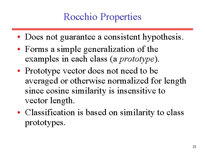
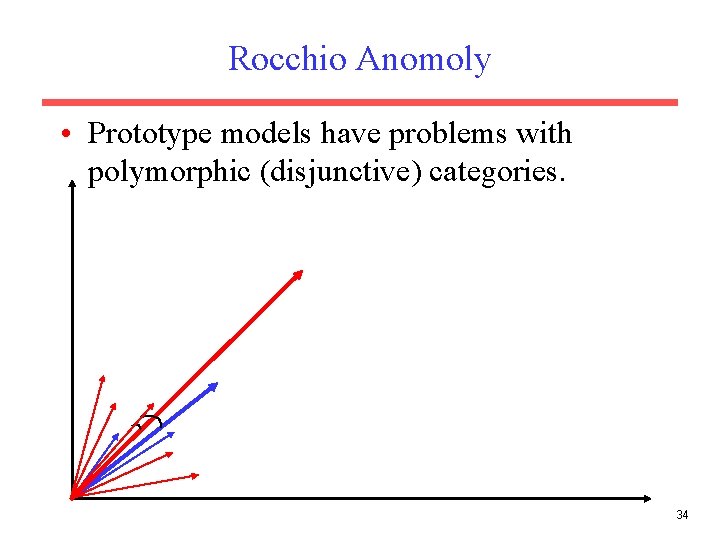
Rocchio Properties • Does not guarantee a consistent hypothesis. • Forms a simple generalization of the examples in each class (a prototype). • Prototype vector does not need to be averaged or otherwise normalized for length since cosine similarity is insensitive to vector length. • Classification is based on similarity to class prototypes. 33

Rocchio Anomoly • Prototype models have problems with polymorphic (disjunctive) categories. 34

Rocchio Time Complexity • Note: The time to add two sparse vectors is proportional to minimum number of non-zero entries in the two vectors. • Training Time: O(|D|(Ld + |Vd|)) = O(|D| Ld) where Ld is the average length of a document in D and Vd is the average vocabulary size for a document in D. • Test Time: O(Lt + |C||Vt|) where Lt is the average length of a test document and |Vt | is the average vocabulary size for a test document. – Assumes lengths of pi vectors are computed and stored during training, allowing cos. Sim(d, pi) to be computed in time proportional to the number of non-zero entries in d (i. e. |Vt|) 35