Text Categorization Categorization Problem Given a universe of

Text Categorization

Categorization Problem: Given a universe of objects and a predefined set of classes, or categories, assign each object to its correct class. l Examples: l Problem Objects Categories Tagging words in context POS tag WSD words in context word sense PP attachment sentences parse trees Language identification text language Text categorization text topic

Overview l Definition of Text Categorization l Techniques – Decision Trees – Maximum Entropy Modeling – k-Nearest Neighbor Classification
 – Task of assigning objects to classes or")
Text categorization l Classification (= Categorization) – Task of assigning objects to classes or categories l Text categorization – Task of classifying the topic or theme of a document

Statistical classification l Training set of objects l Data representation model l Model class l Training procedure l Evaluation

Training set of objects l l A set of objects, each labeled by one or more classes Example from Reuters <REUTERS TOPICS="YES" NEWID="2005"> <DATE> 5 -MAR-1987 09: 22: 57. 75</DATE> <TOPICS><D>earn</D></TOPICS> <PLACES><D>usa</D></PLACES> <TEXT> <TITLE>NORD RESOURCES CORP < NRD> 4 TH QTR NET</TITLE> <DATELINE> DAYTON, Ohio, March 5 - </DATELINE> <BODY>Shr 19 cts vs 13 cts Net 2, 656, 000 vs 1, 712, 000 Revs 15. 4 mln vs 9, 443, 000 Avg shrs 14. 1 mln vs 12. 6 mln Shr 98 cts vs 77 cts Net 13. 8 mln vs 8, 928, 000 Revs 58. 8 mln vs 48. 5 mln Avg shrs 14. 0 mln vs 11. 6 mln NOTE: Shr figures adjusted for 3 -for-2 split paid Feb 6, 1987. Reuter  </BODY></TEXT> </REUTERS>

Data Representation Model l The training set is encoded via a data representation model l Typically, each object in the training set is represented by a pair (x, c), where: – x: a vector of measurements – c: class label

Data Representation l For text categorization: – use words that are frequent in “earnings” documents – the 20 most representative words are: vs, min, cts, loss, &, 000, profit, dlrs, pct, etc. l Each document is represented as vector where and tfij is the number of occurrences of word i in document j and lj is the length of document j. word sij vs 5 mln 5 cts 3 ; 3 & 3 000 4 loss 0 ‘ 0 “ 0 3 4 profit 0 dlrs 3 1 2 pct 0 is 0 that 0 net 3 lt 2 at 0

Model Class and Training Procedure l Model class – A parameterized family of classifiers – e. g. a model class for binary classification: g(x) = w∙x + w 0 • if g(x) > 0, choose class c 1, else c 2 l Training procedure – Algorithm to select one classifier from this family – i. e. , to select proper parameters values (e. g. w, w 0)

Evaluation Borrowing from IR, NLP systems are evaluated by precision, recall, etc. l Example: for text categorization, given a set of documents of which a subset is in a particular category (say, “earnings”), the system classifies some other subset of the documents as belonging to the “earnings” category. l The results of the system are compared with the actual results as follows: l Correct Incorrect Assigned tp (true positive) fp (false positive) Not Assigned fn (false negative) tn (true negative)

Evaluation measures l Precision l Recall l Accuracy l Error

Evaluation of text categorization l macro-averaging – Compute an evaluation measure for each contingency table separately and average over categories – gives equal weight to each category – macro-averaged precision = l micro-averaging – Make a single contingency table for all categories by summing the scores in each cell, then compute the evaluation measure for the whole table – gives equal weight to each object – micro-averaged precision =

Classification Techniques l Naïve Bayes l Decision Trees l Maximum Entropy Modeling l Support Vector Machines l k-Nearest Neighbor

Bayesian Classifiers

Bayesian Methods l l l Learning and classification methods based on probability theory Bayes theorem plays a critical role in probabilistic learning and classification Build a generative model that approximates how data is produced Uses prior probability of each category given no information about an item Categorization produces a posterior probability distribution over the possible categories given a description of an item

Bayes’ Rule prior probability posterior probability

Maximum a posteriori Hypothesis

Maximum likelihood Hypothesis If all hypotheses are a priori equally likely, need only to consider the P(D|h) term:

Naïve Bayes Classifiers Task: Classify a new instance based on a tuple of attribute values
 – Can be estimated from")
Naïve Bayes Classifier: Assumptions l P (c j ) – Can be estimated from the frequency of classes in the training examples. l P(x 1, x 2, …, xn|cj) – O(|X|n • |C|) – Could only be estimated if a very, very large number of training examples was available. Conditional Independence Assumption: Assume that the probability of observing the conjunction of attributes is equal to the product of the individual probabilities.

The Naïve Bayes Classifier Flu X 1 runnynose l X 2 sinus X 3 cough X 4 fever X 5 muscle-ache Conditional Independence Assumption: features are independent of each other given the class:

Learning the Model C X 1 l X 2 X 3 X 4 X 5 X 6 Common practice: maximum likelihood – simply use the frequencies in the data

Problem with Max Likelihood Flu X 1 runnynose X 2 sinus X 3 cough X 4 fever X 5 muscle-ache l What if we have seen no training cases where patient had no flu and muscle aches? l Zero probabilities cannot be conditioned away, no matter the other evidence!

Smoothing to Avoid Overfitting # of values of Xi l Somewhat more subtle version overall fraction in data where Xi=xi, k extent of “smoothing”

Text Classification Using Naïve Bayes: Basic method l l Attributes are text positions, values are words. Naive Bayes assumption is clearly violated. – Example? Still too many possibilities l Assume that classification is independent of the positions of the words – Use same parameters for each position l
 and")
Text Classification Algorithms: Learning From training corpus, extract Vocabulary l Calculate required P(cj) and P(xk | cj) terms l – For each cj in C do • docsj subset of documents for which the target class is cj • • Textj single document containing all docsj • for each word xk in Vocabulary – nk number of occurrences of xk in Textj –

Text Classification Algorithms: Classifying l positions all word positions in current document which contain tokens found in Vocabulary l Return c. NB, where
) Ld is the average")
Naive Bayes Time Complexity l Training Time: O(|D|Ld + |C||V|)) Ld is the average length of a document in D where – Assumes V and all Di , ni, and nij pre-computed in O(|D|Ld) time during one pass through all of the data. – Generally just O(|D|Ld) since usually |C||V| < |D|Ld l Test Time: O(|C| Lt) where Lt is the average length of a test document l Very efficient overall, linearly proportional to the time needed to just read in all the data

Underflow Prevention Multiplying lots of probabilities, which are between 0 and 1 by definition, can result in floating-point underflow l Since log(xy) = log(x) + log(y), it is better to perform all computations by summing logs of probabilities rather than multiplying probabilities l Class with highest final un-normalized log probability score is still the most probable l

Naïve Bayes Posterior Probabilities Classification results of naïve Bayes (the class with maximum posterior probability) are usually fairly accurate l However, due to the inadequacy of the conditional independence assumption, the actual posterior-probability numerical estimates are not l – Output probabilities are generally very close to 0 or 1

Two Models l Model 1: Multivariate binomial – One feature Xw for each word in dictionary – Xw = true in document d if w appears in d – Naive Bayes assumption: • Given the document’s topic, appearance of one word in document tells us nothing about chances that another word appears

Two Models l Model 2: Multinomial – One feature Xi for each word pos in document • feature’s values are all words in dictionary – Value of Xi is the word in position i – Naïve Bayes assumption: • Given the document’s topic, word in one position in document tells us nothing about value of words in other positions – Second assumption: • word appearance does not depend on position for all positions i, j, word w, and class c

Parameter estimation l Binomial model: fraction of documents of topic cj in which word w appears l Multinomial model: fraction of times in which word w appears across all documents of topic cj – creating a mega-document for topic j by concatenating all documents in this topic – use frequency of w in mega-document

Feature selection via Mutual Information We might not want to use all words, but just reliable, good discriminators l In training set, choose k words which best discriminate the categories. l One way is in terms of Mutual Information: l – For each word w and each category c
 For each category we build a list of k")
Feature selection via MI (2) For each category we build a list of k most discriminating terms. l For example (on 20 Newsgroups): l – sci. electronics: circuit, voltage, amp, ground, copy, battery, electronics, cooling, … – rec. autos: car, cars, engine, ford, dealer, mustang, oil, collision, autos, tires, toyota, … Greedy: does not account for correlations between terms l In general feature selection is necessary for binomial NB, but not for multinomial NB l

Evaluating Categorization Evaluation must be done on test data that are independent of the training data (usually a disjoint set of instances). l Classification accuracy: c/n where n is the total number of test instances and c is the number of test instances correctly classified by the system. l Results can vary based on sampling error due to different training and test sets. l Average results over multiple training and test sets (splits of the overall data) for the best results. l

Example: Auto. Yahoo! l Classify 13, 589 Yahoo! webpages in “Science” subtree into 95 different topics (hierarchy depth 2)
 l Classify webpages from CS departments into: – student, faculty,")
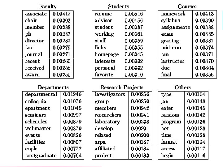
Example: Web. KB (CMU) l Classify webpages from CS departments into: – student, faculty, course, project

Web. KB Experiment l Train on ~5, 000 hand-labeled web pages – Cornell, Washington, U. Texas, Wisconsin l Crawl and classify a new site (CMU) l Results:

NB Model Comparison
")
Sample Learning Curve (Yahoo Science Data)
 attributes A 1,")
Importance of Conditional Independence Assume a domain with 20 binary (true/false) attributes A 1, …, A 20, and two classes c 1 and c 2. Goal: for any case A=A 1, …, A 20 estimate P(A, ci). A) No independence assumptions: Computation of 221 parameters (one for each combination of values) ! l l l The training database will not be so large! Huge Memory requirements / Processing time. Error Prone (small sample error). B) Strongest conditional independence assumptions (all attributes independent given the class) = Naive Bayes: P(A, ci)=P(A 1, ci)P(A 2, ci)…P(A 20, ci) Computation of 20*22 = 80 parameters. l l l Space and time efficient. Robust estimations. What if the conditional independence assumptions do not hold? ? C) More relaxed independence assumptions Tradeoff between A) and B)

Conditions for Optimality of Naïve Bayes Answer Fact Sometimes NB performs well even if the Conditional Independence assumptions are badly violated. Questions Assume two classes c 1 and c 2. A new case A arrives. NB will classify A to c 1 if: P(A, c 1) > P(A, c 2) P(A, c 1) P(A, c 2) Class of A Actual Probability 0. 1 0. 01 c 1 Estimated Probability by NB 0. 08 0. 07 c 1 WHY? And WHEN? Hint Classification is about predicting the correct class label and NOT about accurately estimating probabilities. Despite the big error in estimating the probabilities the classification is still correct. Correct estimation accurate prediction but NOT accurate prediction Correct estimation

Naïve Bayes is Not So Naïve l Naïve Bayes: First and Second place in KDD-CUP 97 competition, among 16 (then) state of the art algorithms Goal: Financial services industry direct mail response prediction model. Predict if the recipient of mail will actually respond to the advertisement – 750, 000 records. l Robust to Irrelevant Features cancel each other without affecting results Instead Decision Trees & Nearest-Neighbor methods can heavily suffer from this. l Very good in Domains with many equally important features Decision Trees suffer from fragmentation in such cases – especially if little data A good dependable baseline for text classification (but not the best)! l Optimal if the Independence Assumptions hold: l – If assumed independence is correct, then it is the Bayes Optimal Classifier for problem l Very Fast: – Learning with one pass over the data; testing linear in the number of attributes, and document collection size l l Low Storage requirements Handles Missing Values
")
Interpretability of Naïve Bayes (From R. Kohavi, Silicon Graphics Mine. Set Evidence Visualizer)

Naïve Bayes Drawbacks Doesn’t do higher order interactions l Typical example: Chess end games l – Each move completely changes the context for the next move – C 4. 5 99. 5 % accuracy : NB 87% accuracy. What if you have BOTH high order interactions AND few training data? l Doesn’t model features that do not equally contribute to distinguishing the classes. l – If few features ONLY mostly determine the class, additional features usually decrease the accuracy. – Because NB gives same weight to all features.

Decision Trees

Decision Trees Example: decision whether to assign documents to the category "earning" node 1 7681 articles P(c|n 1) = 0. 300 split: cts value: 2 cts < 2 cts 2 node 2 5977 articles P(c|n 2) = 0. 116 split: net value: 1 net < 1 node 3 5436 articles P(c|n 3) = 0. 050 node 5 1704 articles P(c|n 5) = 0. 943 split: vs value: 2 net 1 vs < 2 node 4 541 articles P(c|n 4) = 0. 649 node 6 201 articles P(c|n 6) = 0. 694 vs 2 node 7 1403 articles P(c|n 7) = 0. 996
 l Growing a tree with training data –")
Decision Trees - Training procedure (1) l Growing a tree with training data – splitting criterion • for finding the feature and its value on which to split • e. g. maximum information gain – stopping criterion • determines when to stop splitting • e. g. all elements at node have same category l Pruning it back to reasonable size – to avoid overfitting the training set e. g. ‘dlrs’ and ‘pct’ in just one document – to optimize performance
 – H(t|a) = H(t) – (p. LH(t.")
Maximum Information Gain l Information gain H(t) – H(t|a) = H(t) – (p. LH(t. L) + p. RH(t. R)) where: a is attribute we split on t is distribution of the node we split p. L and p. R are the percent of nodes passed on to left and right nodes t. L and t. R are the distributions of left and right nodes l Choose attribute which maximizes IG Example: H(n 1) = - 0. 3 log(0. 3) - 0. 7 log(0. 7) = 0. 881 H(n 2) = 0. 518 H(n 5) = 0. 315 H(n 1) – H(n 1| ‘cts’) = 0. 881 – (5977/7681) · 0. 518 – (1704/7681) · 0. 315 = 0. 408
 At each step, drop a node considered least helpful")
Decision Trees – Pruning (1) At each step, drop a node considered least helpful l Find best tree using validation on validation set l – validation set: portion of training data held out from training l Find best tree using cross-validation – I. Determine the optimal tree size • 1. Divide training data into N partitions • 2. Grow using N-1 partitions, and prune using held-out partition • 3. Repeat 2. N times • 4. Determine average pruned tree size as optimal tree size – II. Training using total training data, and pruning back to optimal size
 l l Effect of pruning on accuracy Optimal performance")
Decision Trees - Pruning (2) l l Effect of pruning on accuracy Optimal performance on test set pruning 951 nodes
")
Decision Trees Summary Useful for non-trivial classification tasks (for simple problems, use simpler methods) l Tend to split the training set into smaller and smaller subsets: l – may lead to poor generalizations – not enough data for reliable prediction – accidental regularities Volatile: very different model from slightly different data l Can be interpreted easily l – easy to trace the path – easy to debug one’s code – easy to understand a new domain

Maximum Entropy Modeling

Maximum Entropy Modeling l Maximum Entropy Modeling – The model with maximum entropy of all the models that satisfy the constraints – desire to preserve as much uncertainty as possible l Model class: log linear model l Training procedure: generalized iterative scaling
 word l Model class: loglinear model – i : weight")
Maximum Entropy Modeling (2) word l Model class: loglinear model – i : weight for i-th feature – Z : normalizing constant l Class of new document – compute p(x, 0), p(x, 1) – choose the class label with the greater probability log(ai) vs 0. 613 mln -0. 110 cts 1. 298 ; -0. 432 & -0. 429 000 -0413 loss -0. 332 ‘ -0. 085 “ 0. 202 3 -0. 463 profit 0. 360 dlrs -0. 202 1 -0. 211 pct -0. 260 is -0. 546 s -0. 490 that -0. 285 net -0. 300 lt 1. 016 at -0. 465 f. K+1 0. 009
 l Training procedure: generalized interative scaling – Expected value of")
Maximum Entropy Modeling (3) l Training procedure: generalized interative scaling – Expected value of p: – Epfi maximum entropy distribution p*: Ep*fi = Epfi l Algorithm 1. initialize (1). compute Epfi. n=1 2. compute p(n)(x, c) for each training data 3. compute Ep(n)fi 4. update (n+1) 5. if converged, stop. otherwise n=n+1, goto 2
 l Define (K+1)th feature: for the constraint that sum of")
Maximum Entropy Modeling (4) l Define (K+1)th feature: for the constraint that sum of fi is equal to C l Expected value of p is defined as l Expected value for the empirical distribution is computed as l Expected value of p is approximately computed as
 1. Initialize {ai(1)}.")
GIS Algorithm (full) 1. Initialize {ai(1)}.
 word l Application to text categorization – trained on 9603")
Maximum Entropy Modeling (6) word l Application to text categorization – trained on 9603 articles, 500 iteration – test result: 88. 6% accuracy log(ai) vs 0. 613 mln -0. 110 cts 1. 298 ; -0. 432 & -0. 429 000 -0413 loss -0. 332 ‘ -0. 085 “ 0. 202 3 -0. 463 profit 0. 360 dlrs -0. 202 1 -0. 211 pct -0. 260 is -0. 546 s -0. 490 that -0. 285 net -0. 300 lt 1. 016 at -0. 465 f. K+1 0. 009
 l Shortcoming of MEM – restricted to binary feature •")
Maximum Entropy Modeling (7) l Shortcoming of MEM – restricted to binary feature • low performance in some situations – computationally expensive: slow convergence – the lack of smoothing can cause problem l Strength of MEM – can specify all possible relevant information • complex features can be defined – can use heterogeneous features and weighting feature – an integrated framework for feature selection & classification • a very large number of features could be down to a manageable size during training procedure

Vector Space Classifiers

Vector Space Representation l Each document is a vector, one component for each term (= word). l Normalize to unit length. l Properties of vector space – terms are axes – n docs live in this space – even with stemming, may have 10, 000+ dimensions, or even 1, 000+
 labeled by its")
Classification Using Vector Spaces l Each training doc a point (vector) labeled by its class l Similarity hypothesis: docs of the same class form a contiguous region of space. Or: Similar documents are usually in the same class. l Define surfaces to delineate classes in space

Classes in a Vector Space Similarity hypothesis true in general? Government Science Arts

Given a Test Document l Figure out which region it lies in l Assign corresponding class

Test Document = Government Science Arts
")
Binary Classification l Consider 2 class problems l How do we define (and find) the separating surface? l How do we test which region a test doc is in?

Separation by Hyperplanes l Assume linear separability for now: – in 2 dimensions, can separate by a line – in higher dimensions, need hyperplanes l Can find separating hyperplane by linear programming (e. g. perceptron): – separator can be expressed as ax + by = c

Linear Programming / Perceptron Find a, b, c, such that ax + by c for red points ax + by c for blue points.

Relationship to Naïve Bayes? Find a, b, c, such that ax + by c for red points ax + by c for blue points.

Linear Classifiers l Many common text classifiers are linear classifiers l Despite this similarity, large performance differences – For separable problems, there is an infinite number of separating hyperplanes. Which one do you choose? – What to do for non-separable problems?

Which Hyperplane? In general, lots of possible solutions for a, b, c

Which Hyperplane? l l Lots of possible solutions for a, b, c. Some methods find a separating hyperplane, but not the optimal one (e. g. , perceptron) Most methods find an optimal separating hyperplane Which points should influence optimality? – All points • Linear regression • Naïve Bayes – Only “difficult points” close to decision boundary • Support vector machines • Logistic regression (kind of)
 l Example features of a linear")
Hyperplane: Example Class: “interest” (as in interest rate) l Example features of a linear classifier (SVM) l wi ti 0. 70 prime 0. 67 rate 0. 63 interest 0. 60 rates 0. 46 discount 0. 43 bundesbank wi ti -0. 71 dlrs -0. 35 world -0. 33 sees -0. 25 year -0. 24 group -0. 24 dlr

More Than Two Classes l One-of classification: each document belongs to exactly one class – How do we compose separating surfaces into regions? l Any-of or multiclassification – For n classes, decompose into n binary problems l Vector space classifiers for one-of classification – Use a set of binary classifiers – Centroid classification – K nearest neighbor classification

Composing Surfaces: Issues ? ? ?

Set of Binary Classifiers Build a separator between each class and its complementary set (docs from all other classes). l Given test doc, evaluate it for membership in each class. l For one-of classification, declare membership in classes for class with: l – maximum score – maximum confidence – maximum probability l Why different from multiclassification?

Negative Examples l Formulate as above, except negative examples for a class are added to its complementary set. Positive examples Negative examples

Centroid Classification l Given training docs for a class, compute their centroid l Now have a centroid for each class l Given query doc, assign to class whose centroid is nearest l Compare to Rocchio

Example Government Science Arts

k-Nearest Neighbor

k Nearest Neighbor Classification l To classify document d into class c l Define k-neighborhood N as k nearest neighbors of d l Count number of documents l in N that belong to c l Estimate P(c|d) as l/k
 P(science| )? Government Science Arts")
Example: k=6 (6 NN) P(science| )? Government Science Arts

Cover and Hart 1967 l Asymptotically, the error rate of 1 - nearest-neighbor classification is less than twice the Bayes rate. l Assume: query point coincides with a training point. l Both query point and training point contribute error -> 2 times Bayes rate l In particular, asymptotic error rate 0 if Bayes rate is 0.

k. NN Classification: Discussion l 1 NN for “earning” – 95. 3% accuracy l KNN Classification – no training – needs effective similarity measure • cosine, Euclidean distance, Value Difference Metric • Performance is very dependent on the right similarity metric – is computationally expensive – is robust and conceptually simple method

k. NN vs. Regression l l l Bias/Variance tradeoff Variance ≈ Capacity k. NN has high variance and low bias. Regression has low variance and high bias. Consider: Is an object a tree? (Burges) Too much capacity/variance, low bias – Botanist who memorizes – Will always say “no” to new object (e. g. , #leaves) l Not enough capacity/variance, high bias – Lazy botanist – Says “yes” if the object is green

k. NN: Discussion Classification time linear in training set l No feature selection necessary l Scales well with large number of classes l – Don’t need to train n classifiers for n classes l Classes can influence each other – Small changes to one class can have ripple effect Scores can be hard to convert to probabilities l No training necessary l – Actually: not true. Why?

Number of Neighbors

Support Vector Machines

Recall: Which Hyperplane? In general, lots of possible solutions for a, b, c. l Support Vector Machine (SVM) finds an optimal solution. l
 SVMs maximize the margin around the separating hyperplane. l The")
Support Vector Machine (SVM) SVMs maximize the margin around the separating hyperplane. l The decision function is fully specified by a subset of training samples, the support vectors. l Quadratic programming problem l Text classification method du jour l Support vectors Maximize margin

Maximum Margin: Formalization w: hyperplane normal l x_i: data point i l y_i: class of data point i (+1 or -1) l l Constraint optimization formalization: l (1) l (2) maximize margin: 2/||w||

Quadratic Programming l One can show that hyperplane w with maximum margin is: i: lagrange multipliers xi: data point i yi: class of data point i (+1 or -1) where the i are the solution to maximizing: Most ai will be zero

Building an SVM Classifier l Now we know how to build a separator for two linearly separable classes l What about classes whose exemplary docs are not linearly separable?

Not Linearly Separable Find a line that penalizes points on “the wrong side”

Penalizing Bad Points Negative for bad points. Define distance for each point with respect to separator ax + by = c: (ax + by) - c for red points c - (ax + by) for blue points.

Solve Quadratic Program l Solution gives “separator” between two classes: choice of a, b l Given a new point (x, y), can score its proximity to each class: – evaluate ax+by – Set confidence threshold 3 5 7

Performance of SVM l l l SVM are seen as best-performing method by many Statistical significance of most results not clear There are many methods that perform about as well as SVM Example: regularized regression (Zhang&Oles) Example of a comparison study: Yang&Liu

Yang&Liu: SVM vs Other Methods

Yang&Liu: Statistical Significance

Yang&Liu: Small Classes
")
Results for Kernels (Joachims)

SVM: Summary l l l SVM have optimal or close to optimal performance Kernels are an elegant and efficient way to map data into a better representation SVM can be expensive to train (quadratic programming) If efficient training is important, and slightly suboptimal performance ok, don’t use SVM For text, linear kernel is common So most SVMs are linear classifiers (like many others), but find a (close to) optimal separating hyperplane
 Model parameters based on small subset (SVs) l Based on")
SVM: Summary (cont. ) Model parameters based on small subset (SVs) l Based on structural risk minimization l l Supports kernel

Resources l l l l l Manning and Schütze. Foundations of Statistical Natural Language Processing. Chapter 16. MIT Press. Trevor Hastie, Robert Tibshirani and Jerome Friedman, "Elements of Statistical Learning: Data Mining, Inference and Prediction" Springer. Verlag, New York. Christopher J. C. Burges. A Tutorial on Support Vector Machines for Pattern Recognition (1998) Data Mining and Knowledge Discovery R. M. Tong, L. A. Appelbaum, V. N. Askman, J. F. Cunningham. Conceptual Information Retrieval using RUBRIC. Proc. ACM SIGIR 247 -253, (1987). S. T. Dumais, Using SVMs for text categorization, IEEE Intelligent Systems, 13(4), Jul/Aug 1998. Yiming Yang, S. Slattery and R. Ghani. A study of approaches to hypertext categorization. Journal of Intelligent Information Systems, Volume 18, Number 2, March 2002. Yiming Yang, Xin Liu. A re-examination of text categorization methods. 22 nd Annual International SIGIR, (1999) Tong Zhang, Frank J. Oles: Text Categorization Based on Regularized Linear Classification Methods. Information Retrieval 4(1): 5 -31 (2001)
- Slides: 107