Large Molecules in Astrophysics Weeds or Flowers Frank

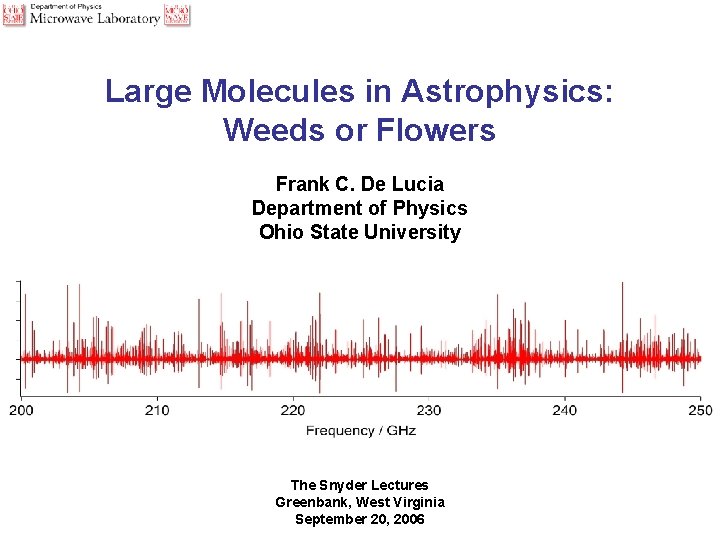
Large Molecules in Astrophysics: Weeds or Flowers Frank C. De Lucia Department of Physics Ohio State University The Snyder Lectures Greenbank, West Virginia September 20, 2006

Lew Snyder: In loco parentis

Lew and Frank Proudly Present The Tool Time Girl

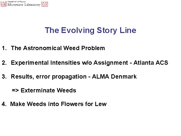
The Evolving Story Line 1. The Astronomical Weed Problem 2. Experimental Intensities w/o Assignment - Atlanta ACS 3. Results, error propagation - ALMA Denmark => Exterminate Weeds 4. Make Weeds into Flowers for Lew

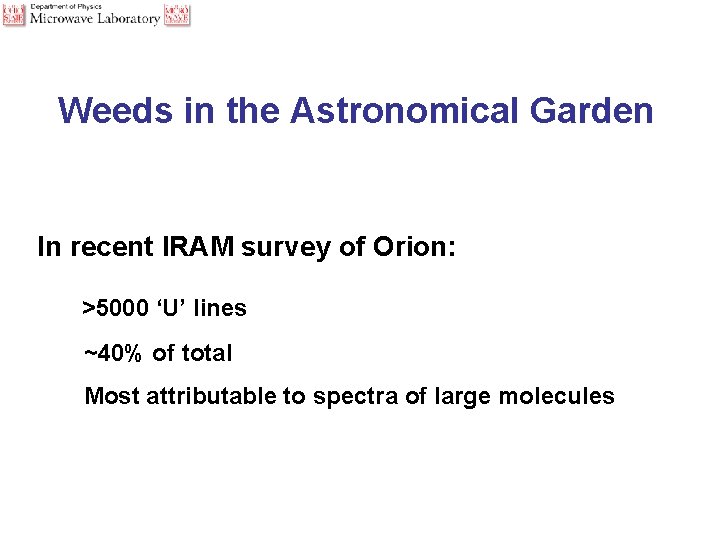
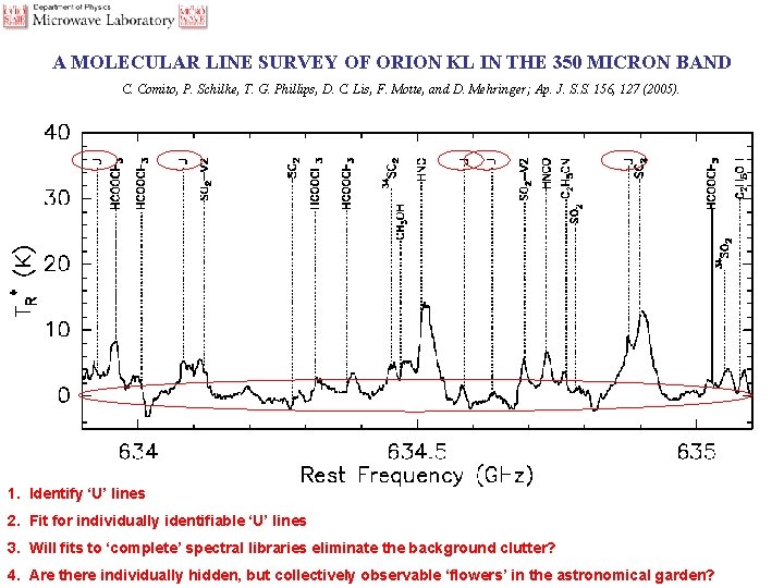
Weeds in the Astronomical Garden In recent IRAM survey of Orion: >5000 ‘U’ lines ~40% of total Most attributable to spectra of large molecules

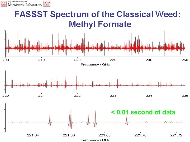
FASSST Spectrum of the Classical Weed: Methyl Formate < 0. 01 second of data

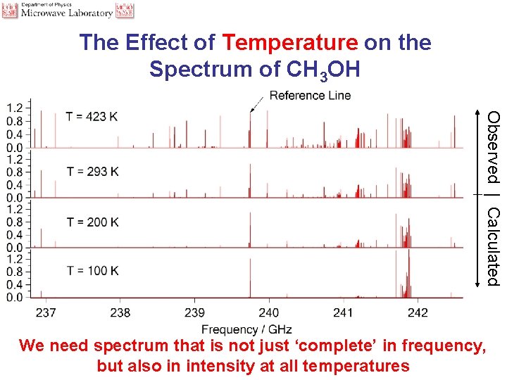
The Effect of Temperature on the Spectrum of CH 3 OH Observed | Calculated We need spectrum that is not just ‘complete’ in frequency, but also in intensity at all temperatures

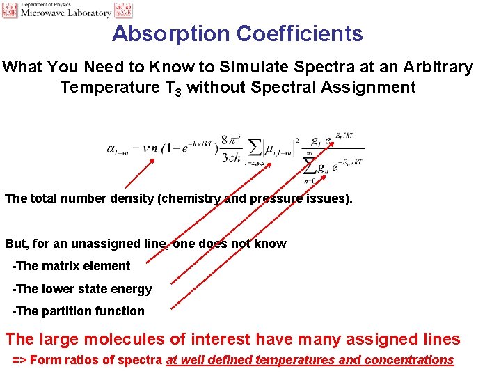
Absorption Coefficients What You Need to Know to Simulate Spectra at an Arbitrary Temperature T 3 without Spectral Assignment The total number density (chemistry and pressure issues). But, for an unassigned line, one does not know -The matrix element -The lower state energy -The partition function The large molecules of interest have many assigned lines => Form ratios of spectra at well defined temperatures and concentrations

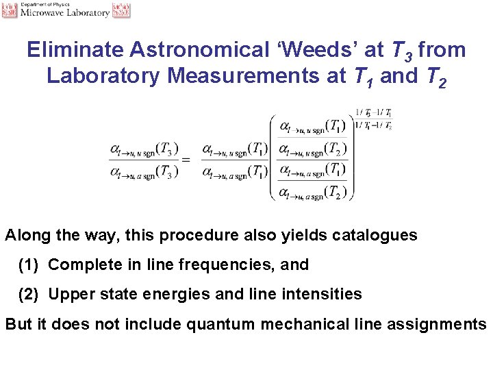
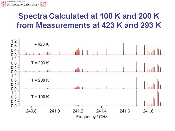
Eliminate Astronomical ‘Weeds’ at T 3 from Laboratory Measurements at T 1 and T 2 Along the way, this procedure also yields catalogues (1) Complete in line frequencies, and (2) Upper state energies and line intensities But it does not include quantum mechanical line assignments

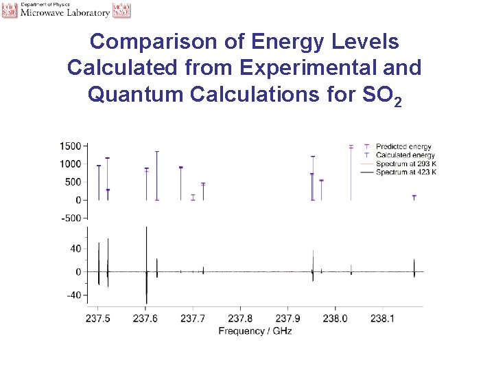
Comparison of Energy Levels Calculated from Experimental and Quantum Calculations for SO 2

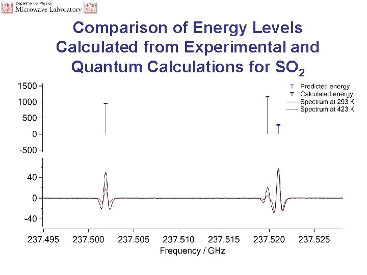
Comparison of Energy Levels Calculated from Experimental and Quantum Calculations for SO 2

Spectra Calculated at 100 K and 200 K from Measurements at 423 K and 293 K

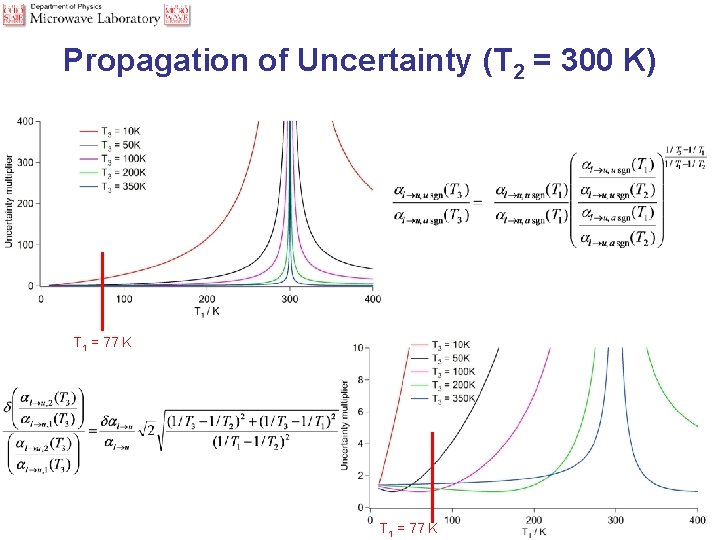
Propagation of Uncertainty (T 2 = 300 K) T 1 = 77 K

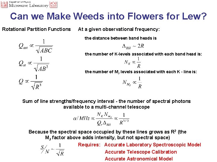
Can we Make Weeds into Flowers for Lew? Rotational Partition Functions At a given observational frequency: the distance between band heads is the number of K-levels associated with each band head is: the number of MJ levels associated with each K - line is: Sum of line strengths/frequency interval - the number of spectral photons available to a multi-channel telescope Because the spectral space occupied by these lines grows as R 2 (the MJ factor above adds intensity, but not spectral space) Requires: Accurate Laboratory Spectroscopic Model Accurate Telescope Calibration Accurate Astronomical Model

A MOLECULAR LINE SURVEY OF ORION KL IN THE 350 MICRON BAND C. Comito, P. Schilke, T. G. Phillips, D. C. Lis, F. Motte, and D. Mehringer; Ap. J. S. S. 156, 127 (2005). 1. Identify ‘U’ lines 2. Fit for individually identifiable ‘U’ lines 3. Will fits to ‘complete’ spectral libraries eliminate the background clutter? 4. Are there individually hidden, but collectively observable ‘flowers’ in the astronomical garden?

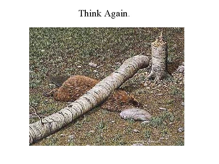
• You've carefully thought out all the angles. • You've done it a thousand times. • It comes naturally to you. • You know what you're doing, its what you've been trained to do your whole life. • Nothing could possibly go wrong, right ?

Think Again.

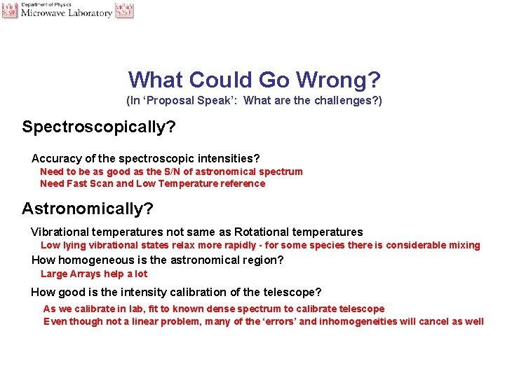
What Could Go Wrong? (In ‘Proposal Speak’: What are the challenges? ) Spectroscopically? Accuracy of the spectroscopic intensities? Need to be as good as the S/N of astronomical spectrum Need Fast Scan and Low Temperature reference Astronomically? Vibrational temperatures not same as Rotational temperatures Low lying vibrational states relax more rapidly - for some species there is considerable mixing How homogeneous is the astronomical region? Large Arrays help a lot How good is the intensity calibration of the telescope? As we calibrate in lab, fit to known dense spectrum to calibrate telescope Even though not a linear problem, many of the ‘errors’ and inhomogeneities will cancel as well

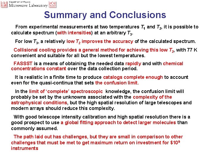
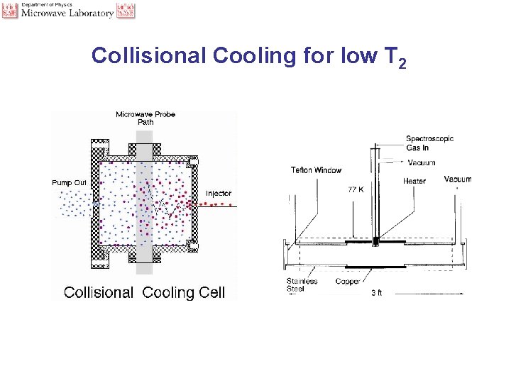
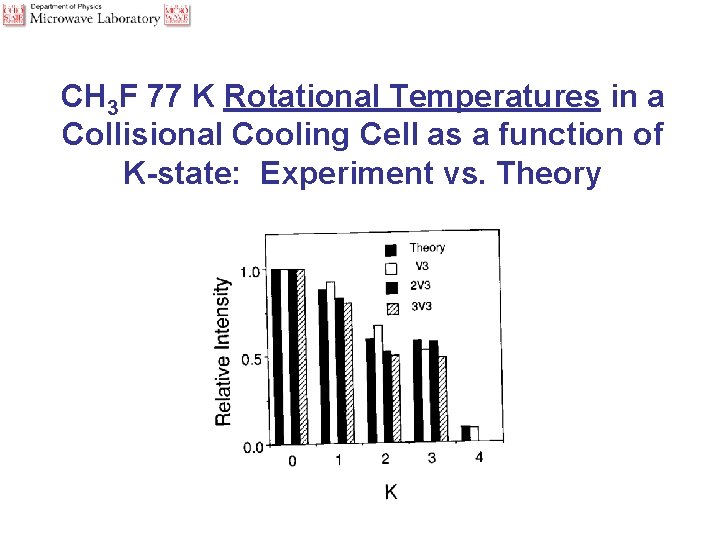
Summary and Conclusions From experimental measurements at two temperatures T 1 and T 2, it is possible to calculate spectrum (with intensities) at an arbitrary T 3. For low T 3, a relatively low T 2 improves the accuracy of the calculated spectrum. Collisional cooling provides a general method for achieving this low T 2, with 77 K convenient and suitable for all but the lowest temperatures. FASSST is a means of obtaining the needed data rapidly and with chemical concentrations constant over the data collection period. It is realistic in a finite time to produce catalogs complete enough to account even for the quasi-continua that sets the confusion limit. In the limit of ‘complete’ spectroscopic knowledge, the confusion limit will probably be set by the unknowns associated with the complexity of the astrophysical conditions, but the high spatial resolution of large telescopes and modern arrays should reduce this complexity. With good telescope intensity calibration and high spatial resolution there is a good prospect to use a global fitting approach to detect larger molecules than commonly assumed. The path laid out has challenges, but they are small in comparison to other challenges that must be met to get maximum return on investment for $10 9 instruments

Abstract Unidentified features in interstellar spectra (‘U’ lines) have persisted almost from the beginning of molecular astrophysics. In recent years, the number of such lines has rapidly increased in parallel with the sensitivity and frequency range of new observational facilities. Initially, the ‘U’ lines often were from ‘exotic’ species, such as HCO+, but now the origins of these unidentified ‘weeds’ are overwhelmingly from previously observed large molecules with dense spectra. The origin of the ‘weeds’ problem lies in the nature of the spectroscopic approach that has typically been used in the millimeter and submillimeter spectral region: the bootstrap narrow-band-observation, assignment, and theoretical prediction cycle. Unfortunately, the ‘weeds’ arise from complex spectra involving many low lying and often interacting vibrational states that are not typically part of the bootstrap process. This talk discusses a purely experimental approach to this problem that does not require spectra assignment but rather relies on the observation of ‘complete’ spectra over a range of temperatures. It also discusses the potential for the use of these ‘complete’ spectra in conjunction with the multiplex capabilities of modern radio telescopes for the detection of large species whose spectra consists of many relatively weak and ordinarily unobservable lines. This approach is enabled by the FASSST spectroscopic system and the use of Collisional Cooling cells to provide reference spectra at low temperature.

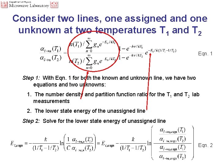
Consider two lines, one assigned and one unknown at two temperatures T 1 and T 2 Eqn. 1 Step 1: With Eqn. 1 for both the known and unknown line, we have two equations and two unknowns: 1. The number density and partition function ratio for the T 1 and T 2 lab measurements 2. The lower state energy of the unassigned line Step 2: Solve for the lower state energy of unassigned line Eqn. 2

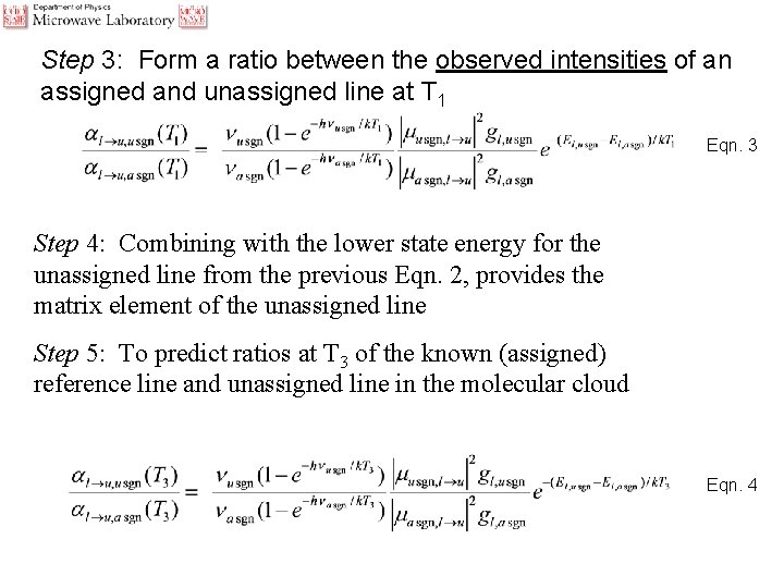
Step 3: Form a ratio between the observed intensities of an assigned and unassigned line at T 1 Eqn. 3 Step 4: Combining with the lower state energy for the unassigned line from the previous Eqn. 2, provides the matrix element of the unassigned line Step 5: To predict ratios at T 3 of the known (assigned) reference line and unassigned line in the molecular cloud Eqn. 4

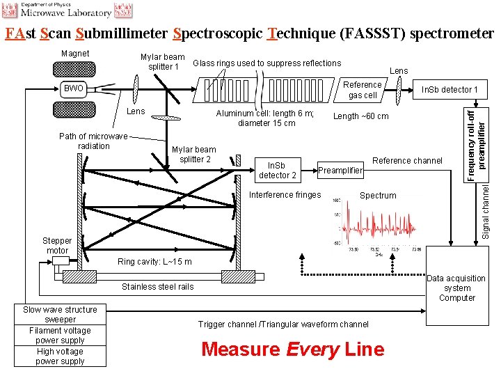
FAst Scan Submillimeter Spectroscopic Technique (FASSST) spectrometer Glass rings used to suppress reflections Lens Reference gas cell BWO Lens Path of microwave radiation Aluminum cell: length 6 m; diameter 15 cm Mylar beam splitter 2 In. Sb detector 1 Length ~60 cm Reference channel Preamplifier Interference fringes Spectrum Stepper motor Signal channel Mylar beam splitter 1 Frequency roll-off preamplifier Magnet Ring cavity: L~15 m Data acquisition system Computer Stainless steel rails Slow wave structure sweeper Filament voltage power supply High voltage power supply Trigger channel /Triangular waveform channel Measure Every Line

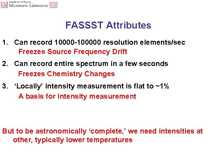
FASSST Attributes 1. Can record 10000 -100000 resolution elements/sec Freezes Source Frequency Drift 2. Can record entire spectrum in a few seconds Freezes Chemistry Changes 3. ‘Locally’ intensity measurement is flat to ~1% A basis for intensity measurement But to be astronomically ‘complete, ’ we need intensities at other, typically lower temperatures

Collisional Cooling for low T 2

CH 3 F 77 K Rotational Temperatures in a Collisional Cooling Cell as a function of K-state: Experiment vs. Theory