JMP DISCOVERY TUSCON 2019 What to Do When

JMP DISCOVERY TUSCON 2019 What to Do When Your Data is a Curve Sam Gardner Principal Research Scientist Elanco Animal Health © 2019 Elanco or its affiliates

Introduction © 2019 Elanco or its affiliates

When is Data a Curve? • For this presentation, I am defining a curve as continuous data recorded over time • Many situations in pharmaceutical research and development generate curves as the data of interest – – Kinetic reaction data Dissolution profiles Continuous process monitoring data Plus many, many more © 2019 Elanco or its affiliates 3

Ways to deal with data that is a curve • Time Aligned – Slice the data (e. g. treat each time point independently) – Use time as a regressor in a prediction model • Use non-parametric smoothing models (e. g. function data analysis) • Use a parametric model based on theory (e. g. nonlinear models) © 2019 Elanco or its affiliates 4

Predicting Dissolution Profiles Time-Aligned Data © 2019 Elanco or its affiliates 5

Dissolution • Dissolution is an in-vitro method that measures the release of the active drug from the drug product into solution. • It is intended to be a surrogate measurement of the in-vivo release of the drug into the patient body system • Dissolution measured at 1 or 2 time points is typically considered a critical quality attribute for solid oral dosage forms (tablets) • Comparison of the rate of release between a reference dissolution profile/curve (e. g. from a clinical trial batch) with a test curve is also commonly performed (e. g. from a scale-up validation batch) (see https: //community. jmp. com/t 5/Discovery-Summit-Europe-2018/Multivariate-Testing-of-the-Similarity-of-Dissolution-Curves/ta-p/51280 for a nice description of this kind of testing ) © 2019 Elanco or its affiliates 6

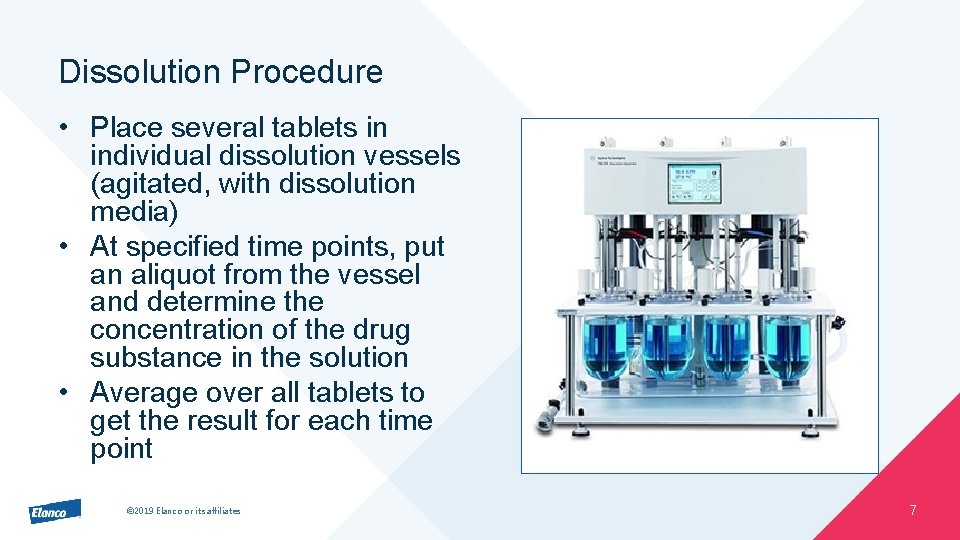
Dissolution Procedure • Place several tablets in individual dissolution vessels (agitated, with dissolution media) • At specified time points, put an aliquot from the vessel and determine the concentration of the drug substance in the solution • Average over all tablets to get the result for each time point © 2019 Elanco or its affiliates 7

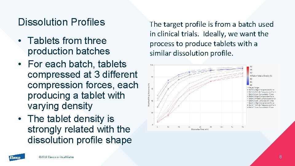
Dissolution Profiles • Tablets from three production batches • For each batch, tablets compressed at 3 different compression forces, each producing a tablet with varying density • The tablet density is strongly related with the dissolution profile shape © 2019 Elanco or its affiliates The target profile is from a batch used in clinical trials. Ideally, we want the process to produce tablets with a similar dissolution profile. 8

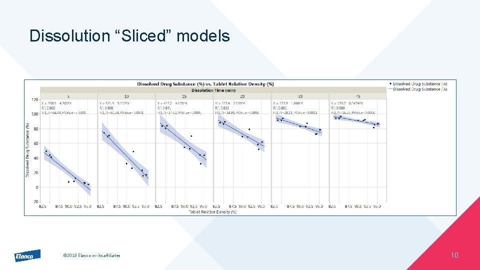
Predicting Dissolution • Approach 1: – Because the data is aligned in time, we can “slice” the curves – For each time point, fit a prediction model for dissolution=f(density) © 2019 Elanco or its affiliates 9

Dissolution “Sliced” models © 2019 Elanco or its affiliates 10

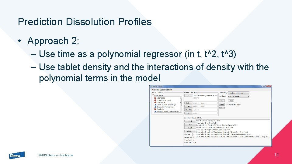
Prediction Dissolution Profiles • Approach 2: – Use time as a polynomial regressor (in t, t^2, t^3) – Use tablet density and the interactions of density with the polynomial terms in the model © 2019 Elanco or its affiliates 11

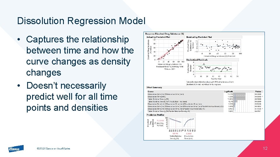
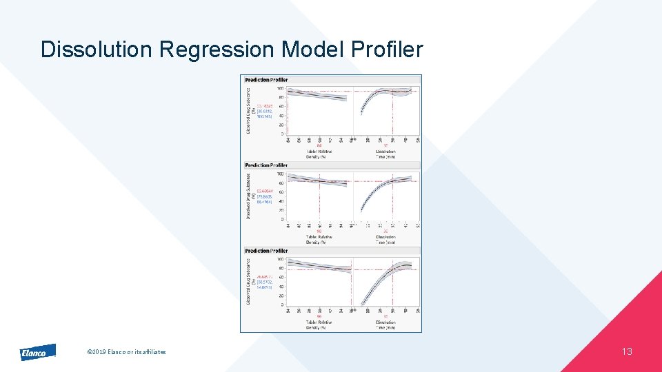
Dissolution Regression Model • Captures the relationship between time and how the curve changes as density changes • Doesn’t necessarily predict well for all time points and densities © 2019 Elanco or its affiliates 12

Dissolution Regression Model Profiler © 2019 Elanco or its affiliates 13

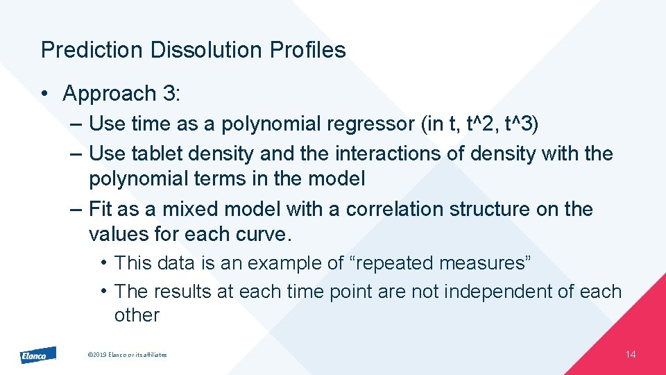
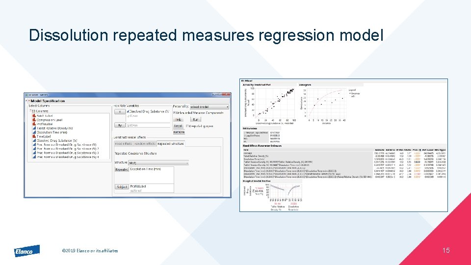
Prediction Dissolution Profiles • Approach 3: – Use time as a polynomial regressor (in t, t^2, t^3) – Use tablet density and the interactions of density with the polynomial terms in the model – Fit as a mixed model with a correlation structure on the values for each curve. • This data is an example of “repeated measures” • The results at each time point are not independent of each other © 2019 Elanco or its affiliates 14

Dissolution repeated measures regression model © 2019 Elanco or its affiliates 15

What’s good and what’s bad about these approaches • Good – Easy to understand the approaches and within the reach of many JMP users – Approach 1 can be one with Fit Y By X/Bivariate – Approach 2 with Fit Least Squares – Approch 3 with JMP Pro/Fit Mixed © 2019 Elanco or its affiliates • Bad – Models are all approximations – May not interpolate or extrapolate well – Doesn’t necessarily predict well everywhere – We probably don’t have the “real” model for the curve 16

Predicting Deuterium Exchange in Lyophilized Monoclonal Antibodies Reduce the Curve Using a Parametric Model © 2019 Elanco or its affiliates 17

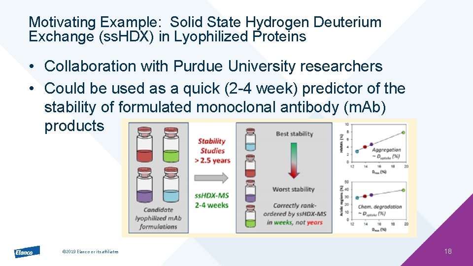
Motivating Example: Solid State Hydrogen Deuterium Exchange (ss. HDX) in Lyophilized Proteins • Collaboration with Purdue University researchers • Could be used as a quick (2 -4 week) predictor of the stability of formulated monoclonal antibody (m. Ab) products © 2019 Elanco or its affiliates 18

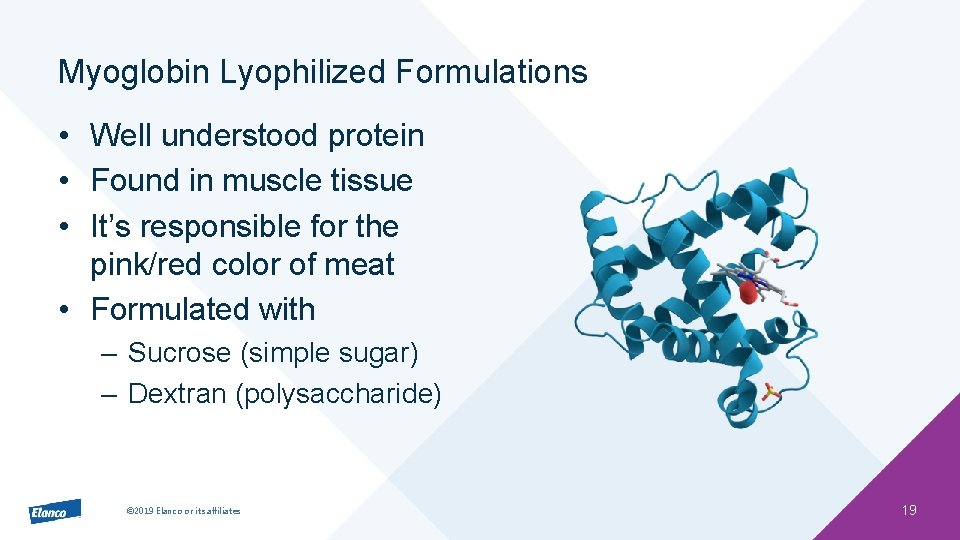
Myoglobin Lyophilized Formulations • Well understood protein • Found in muscle tissue • It’s responsible for the pink/red color of meat • Formulated with – Sucrose (simple sugar) – Dextran (polysaccharide) © 2019 Elanco or its affiliates 19

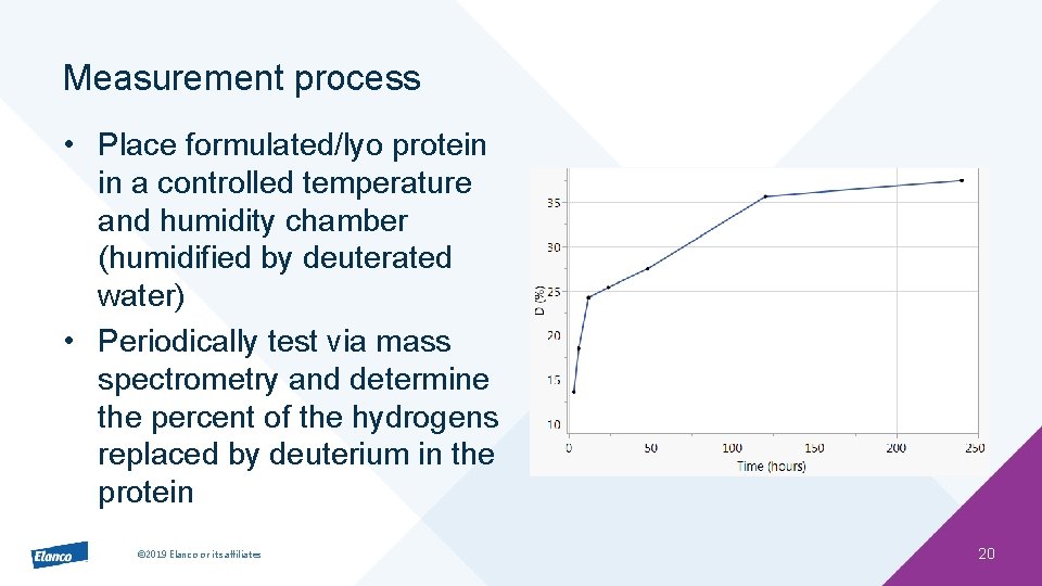
Measurement process • Place formulated/lyo protein in a controlled temperature and humidity chamber (humidified by deuterated water) • Periodically test via mass spectrometry and determine the percent of the hydrogens replaced by deuterium in the protein © 2019 Elanco or its affiliates 20

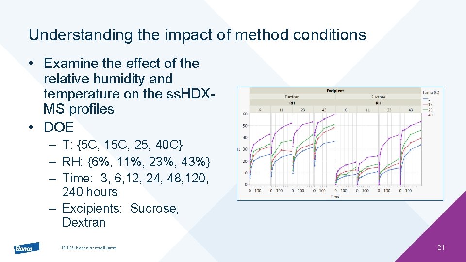
Understanding the impact of method conditions • Examine the effect of the relative humidity and temperature on the ss. HDXMS profiles • DOE – T: {5 C, 15 C, 25, 40 C} – RH: {6%, 11%, 23%, 43%} – Time: 3, 6, 12, 24, 48, 120, 240 hours – Excipients: Sucrose, Dextran © 2019 Elanco or its affiliates 21

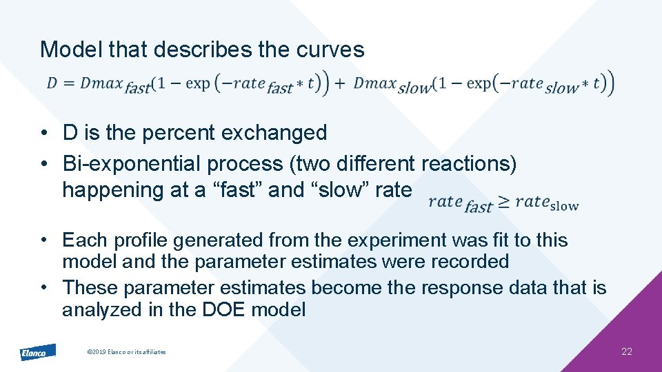
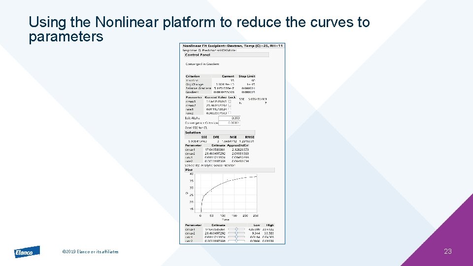
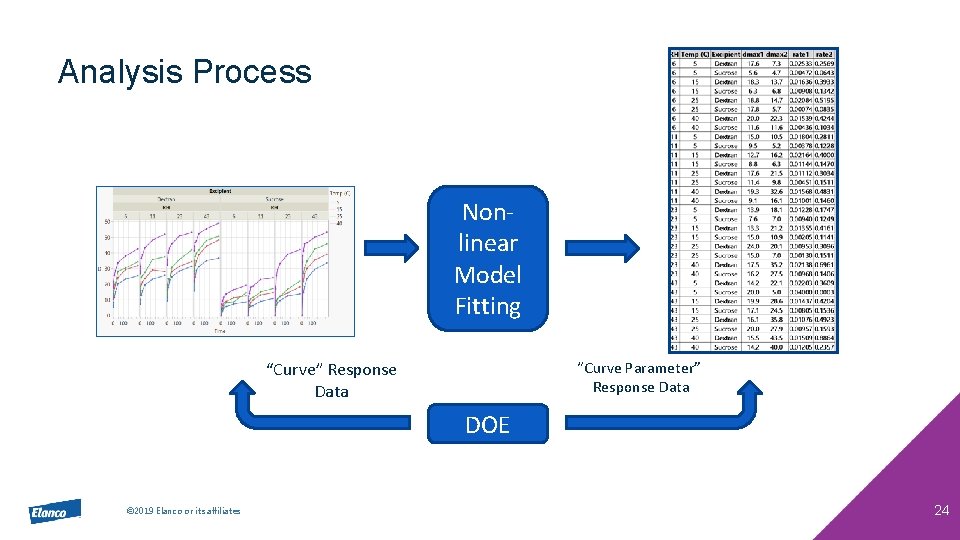
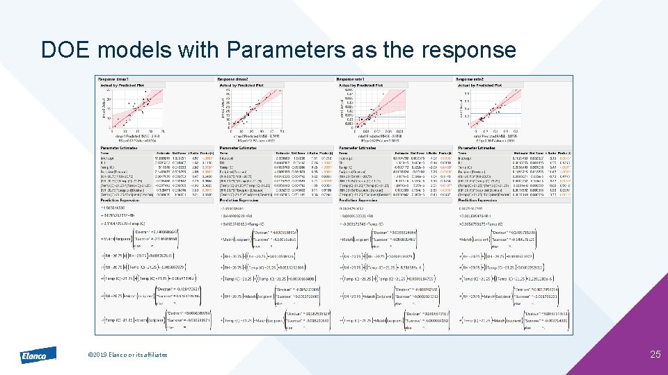
Model that describes the curves • D is the percent exchanged • Bi-exponential process (two different reactions) happening at a “fast” and “slow” rate • Each profile generated from the experiment was fit to this model and the parameter estimates were recorded • These parameter estimates become the response data that is analyzed in the DOE model © 2019 Elanco or its affiliates 22

Using the Nonlinear platform to reduce the curves to parameters © 2019 Elanco or its affiliates 23

Analysis Process Nonlinear Model Fitting “Curve” Response Data “Curve Parameter” Response Data DOE © 2019 Elanco or its affiliates 24

DOE models with Parameters as the response © 2019 Elanco or its affiliates 25

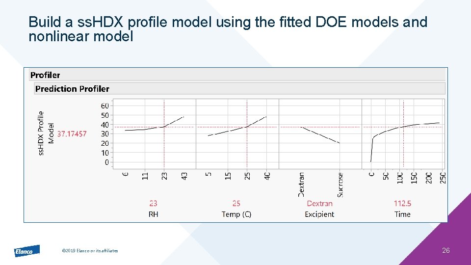
Build a ss. HDX profile model using the fitted DOE models and nonlinear model © 2019 Elanco or its affiliates 26

Predicting High Shear Wet Granulation Power Consumption Profiles Use Functional Data Analysis to Reduce the Curve © 2019 Elanco or its affiliates 27

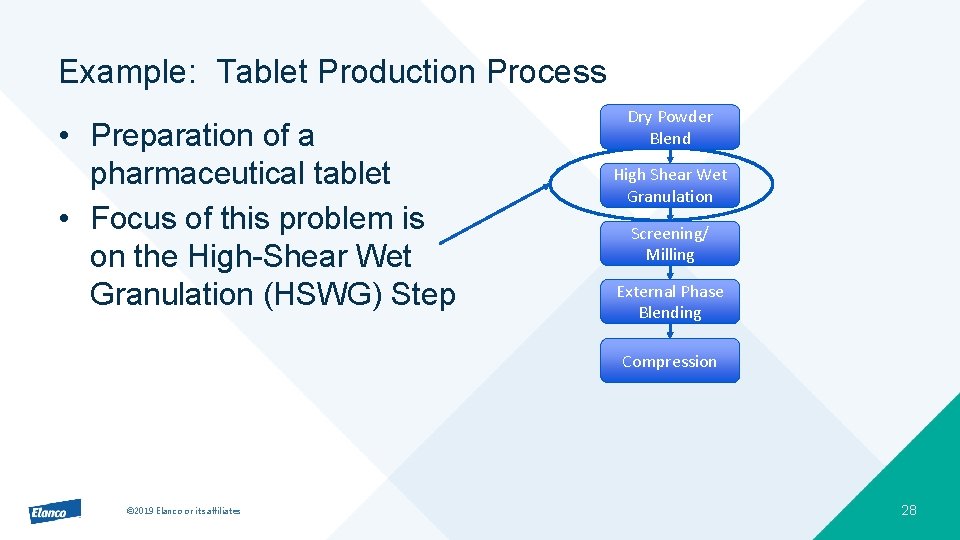
Example: Tablet Production Process • Preparation of a pharmaceutical tablet • Focus of this problem is on the High-Shear Wet Granulation (HSWG) Step Dry Powder Blend High Shear Wet Granulation Screening/ Milling External Phase Blending Compression © 2019 Elanco or its affiliates 28

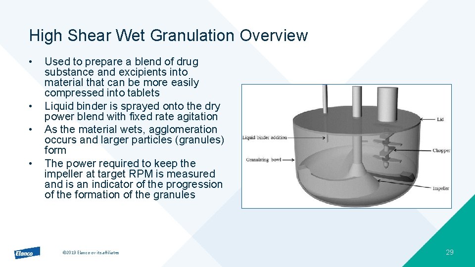
High Shear Wet Granulation Overview • • Used to prepare a blend of drug substance and excipients into material that can be more easily compressed into tablets Liquid binder is sprayed onto the dry power blend with fixed rate agitation As the material wets, agglomeration occurs and larger particles (granules) form The power required to keep the impeller at target RPM is measured and is an indicator of the progression of the formation of the granules © 2019 Elanco or its affiliates 29

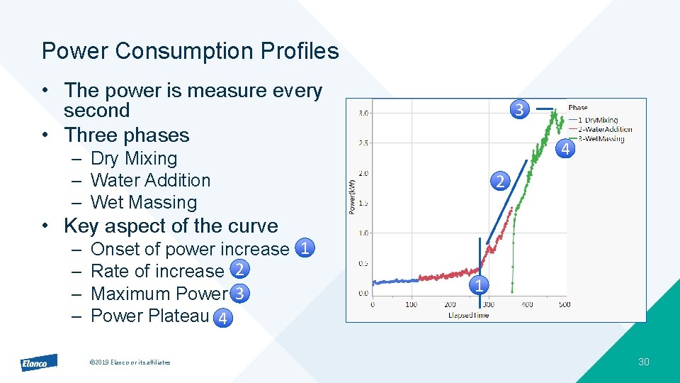
Power Consumption Profiles • The power is measure every second • Three phases 3 4 – Dry Mixing – Water Addition – Wet Massing 2 • Key aspect of the curve – – Onset of power increase 1 Rate of increase 2 Maximum Power 3 Power Plateau 4 © 2019 Elanco or its affiliates 1 30

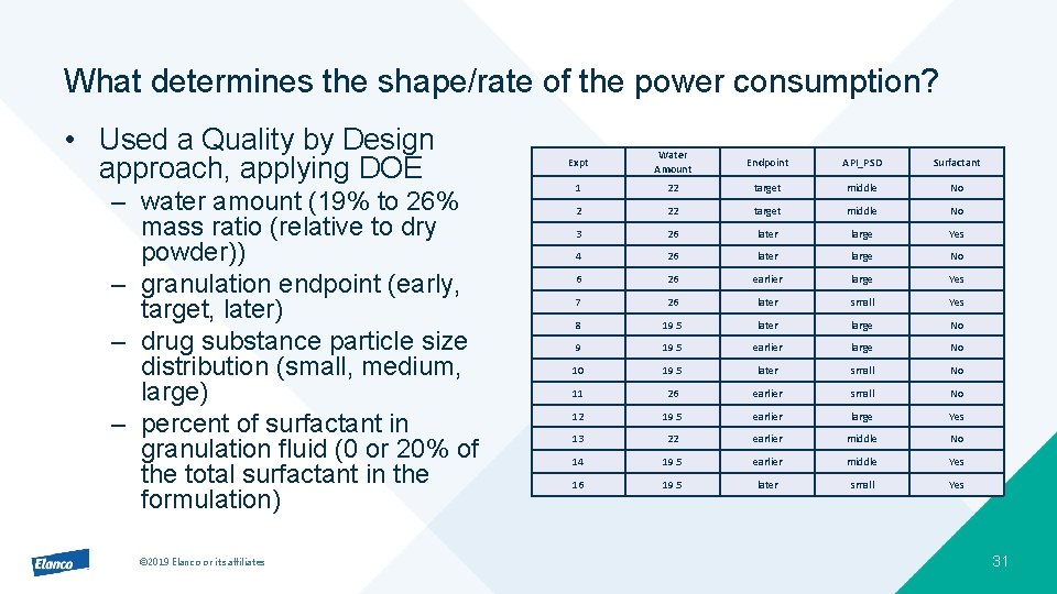
What determines the shape/rate of the power consumption? • Used a Quality by Design approach, applying DOE – water amount (19% to 26% mass ratio (relative to dry powder)) – granulation endpoint (early, target, later) – drug substance particle size distribution (small, medium, large) – percent of surfactant in granulation fluid (0 or 20% of the total surfactant in the formulation) © 2019 Elanco or its affiliates Expt Water Amount Endpoint API_PSD Surfactant 1 22 target middle No 2 22 target middle No 3 26 later large Yes 4 26 later large No 6 26 earlier large Yes 7 26 later small Yes 8 19. 5 later large No 9 19. 5 earlier large No 10 19. 5 later small No 11 26 earlier small No 12 19. 5 earlier large Yes 13 22 earlier middle No 14 19. 5 earlier middle Yes 16 19. 5 later small Yes 31

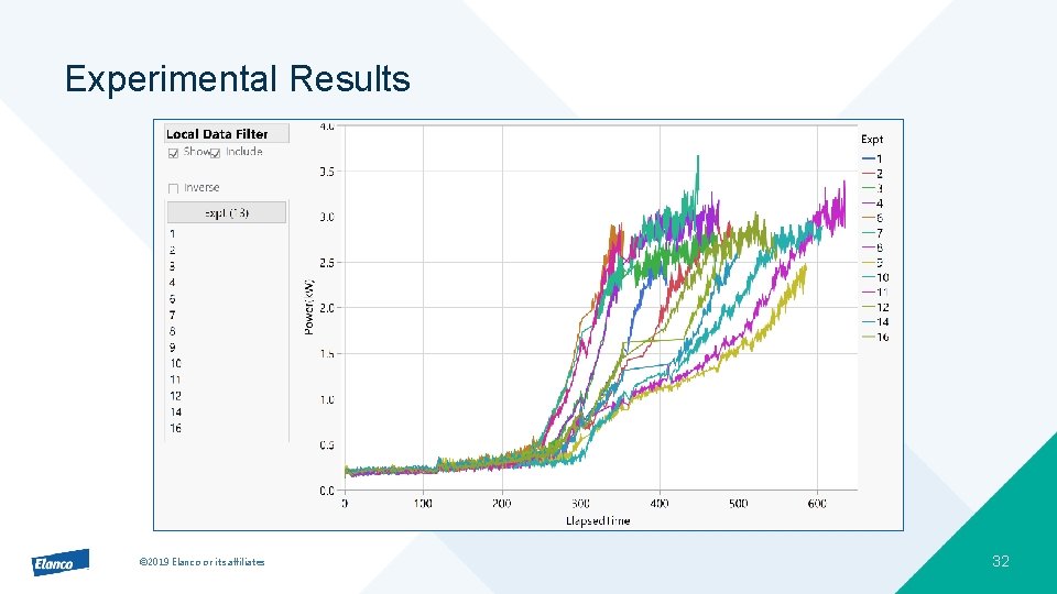
Experimental Results © 2019 Elanco or its affiliates 32

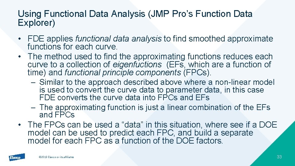
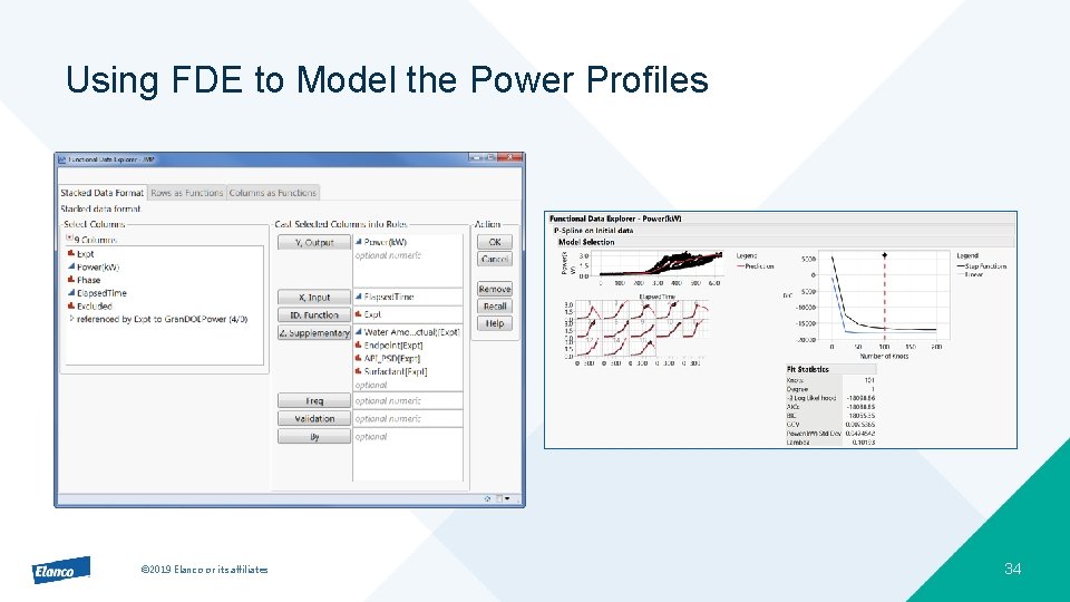
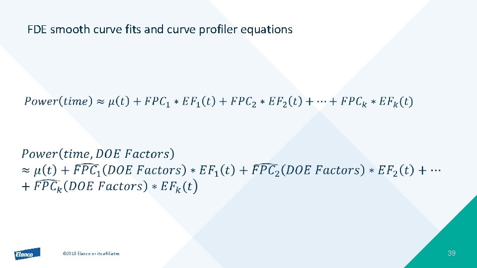
Using Functional Data Analysis (JMP Pro’s Function Data Explorer) • FDE applies functional data analysis to find smoothed approximate functions for each curve. • The method used to find the approximating functions reduces each curve to a collection of eigenfuctions (EFs, which are a function of time) and functional principle components (FPCs). – Similar to the approach described above where a non-linear model is used to convert the curve data to parameter data, in this case FDE converts the curve data into FPCs and EFs – The approximating function is just a linear combination of the EFs and FPCs • The FPCs can be used a “data” in this situation, where see if a DOE model can be used to predict each FPC, and build a separate model for each FPC as a function of the DOE factors. © 2019 Elanco or its affiliates 33

Using FDE to Model the Power Profiles © 2019 Elanco or its affiliates 34

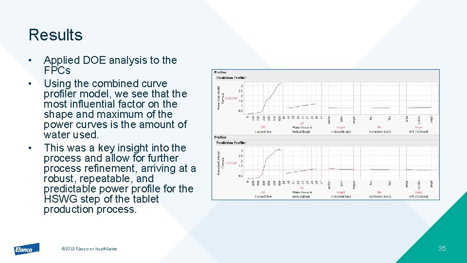
Results • • • Applied DOE analysis to the FPCs Using the combined curve profiler model, we see that the most influential factor on the shape and maximum of the power curves is the amount of water used. This was a key insight into the process and allow for further process refinement, arriving at a robust, repeatable, and predictable power profile for the HSWG step of the tablet production process. © 2019 Elanco or its affiliates 35

Conclusion © 2019 Elanco or its affiliates 36

So, What to Do When Your Data is a Curve? • Apply Simple Approaches of Time Slicing and Regression • Reduce the curve to parameters by fitting the “true” model to each curve • Reduce the curve to parameters from smooth curve models and apply functional data analysis. – If the curves were generated as part of a DOE, use the model parameter estimates as the response data for the DOE. © 2019 Elanco or its affiliates 37

Extra Information © 2019 Elanco or its affiliates 38

FDE smooth curve fits and curve profiler equations © 2019 Elanco or its affiliates 39