Investments CHAPTER 6 7 Cover image Risk Aversion

Investments CHAPTER 6 & 7 Cover image Risk Aversion and Capital Allocation to Risky Assets Slides by Richard D. Johnson Mc. Graw-Hill/Irwin Copyright © 2008 by The Mc. Graw-Hill Companies, Inc. All rights reserved

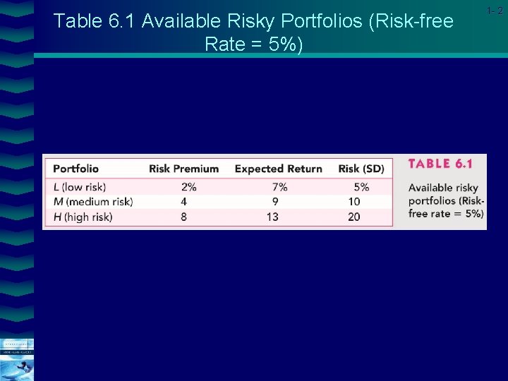
Table 6. 1 Available Risky Portfolios (Risk-free Rate = 5%) Cover image 1 - 2

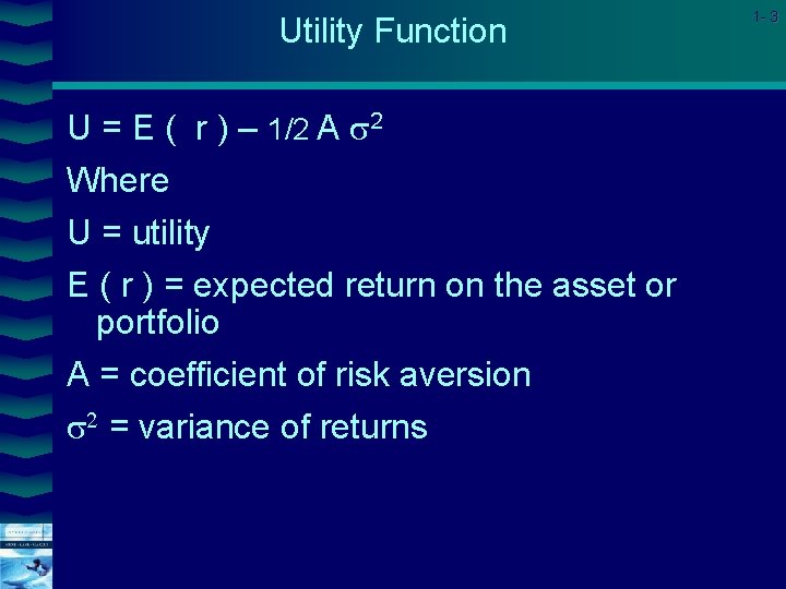
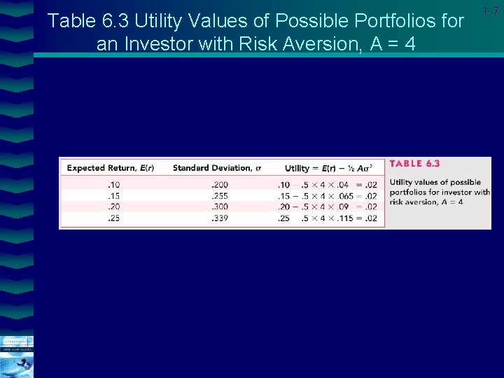
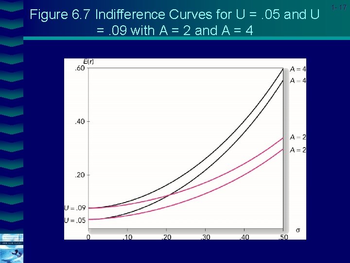
Utility Function U = E ( r ) – 1/2 A 2 Where U = utility E ( r ) = expected return on the asset or portfolio A = coefficient of risk aversion 2 = variance of returns Cover image 1 - 3

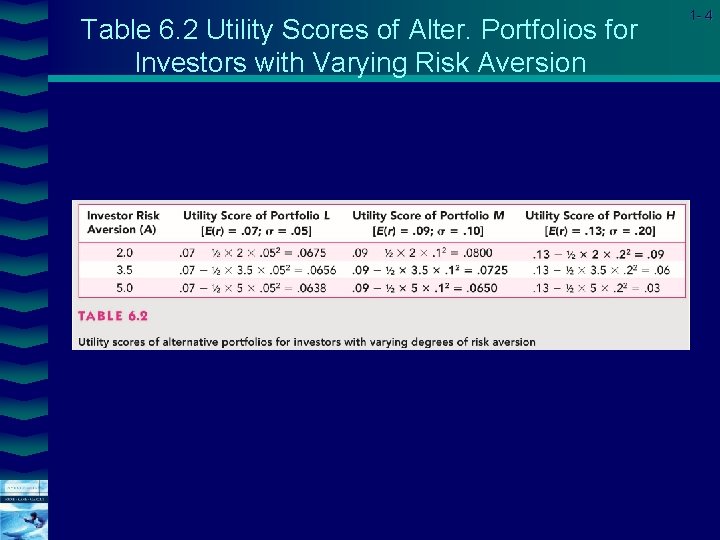
Table 6. 2 Utility Scores of Alter. Portfolios for Investors with Varying Risk Aversion Cover image 1 - 4

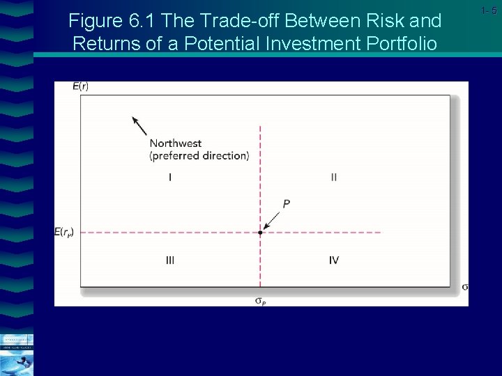
Figure 6. 1 The Trade-off Between Risk and Returns of a Potential Investment Portfolio Cover image 1 - 5

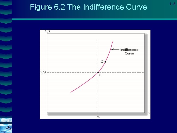
Figure 6. 2 The Indifference Curve Cover image 1 - 6

Table 6. 3 Utility Values of Possible Portfolios for an Investor with Risk Aversion, A = 4 Cover image 1 - 7

Allocating Capital: Risky & Risk Free Assets Ø It’s possible to split investment funds between safe and risky assets. Ø Risk free asset: proxy; T-bills Ø Risky asset: stock (or a portfolio) Cover image 1 - 8

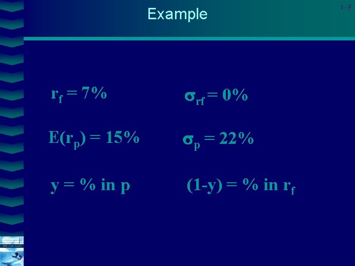
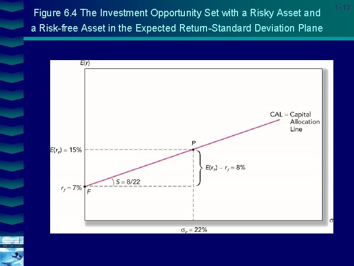
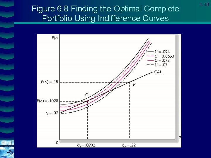
Example Cover image rf = 7% rf = 0% E(rp) = 15% p = 22% y = % in p (1 -y) = % in rf 1 - 9

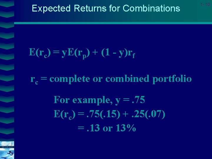
Expected Returns for Combinations E(rc) = y. E(rp) + (1 - y)rf rc = complete or combined portfolio For example, y =. 75 E(rc) =. 75(. 15) +. 25(. 07) =. 13 or 13% Cover image 1 - 10

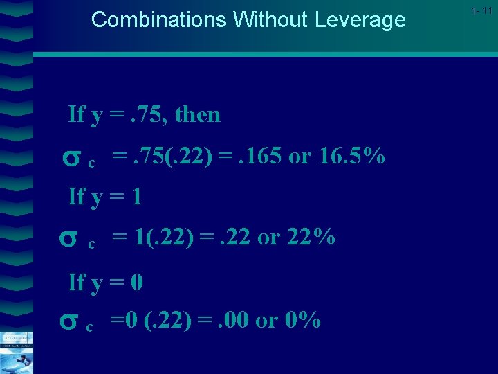
Combinations Without Leverage If y =. 75, then c =. 75(. 22) =. 165 or 16. 5% If y = 1 c = 1(. 22) =. 22 or 22% If y = 0 c =0 (. 22) =. 00 or 0% Cover image 1 - 11

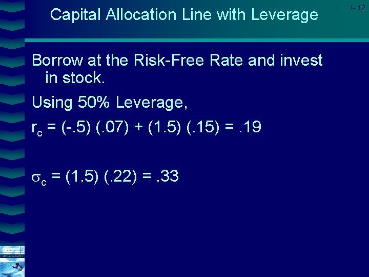
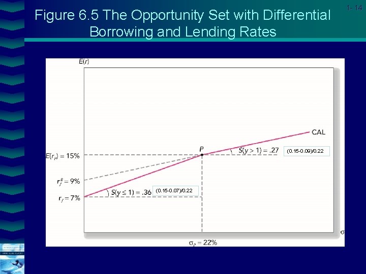
Capital Allocation Line with Leverage Borrow at the Risk-Free Rate and invest in stock. Using 50% Leverage, rc = (-. 5) (. 07) + (1. 5) (. 15) =. 19 c = (1. 5) (. 22) =. 33 Cover image 1 - 12

Figure 6. 4 The Investment Opportunity Set with a Risky Asset and a Risk-free Asset in the Expected Return-Standard Deviation Plane Cover image 1 - 13

Figure 6. 5 The Opportunity Set with Differential Borrowing and Lending Rates (0. 15 -0. 09)/0. 22 (0. 15 -0. 07)/0. 22 Cover image 1 - 14

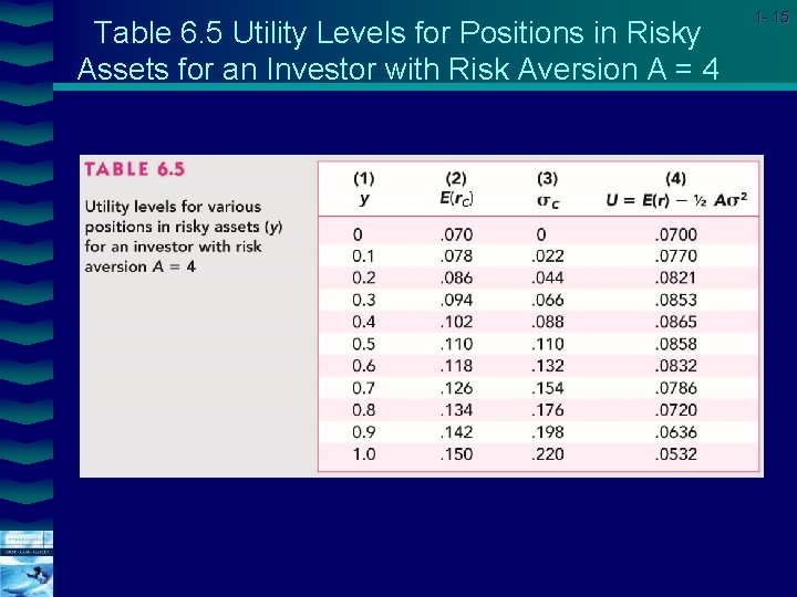
Table 6. 5 Utility Levels for Positions in Risky Assets for an Investor with Risk Aversion A = 4 Cover image 1 - 15

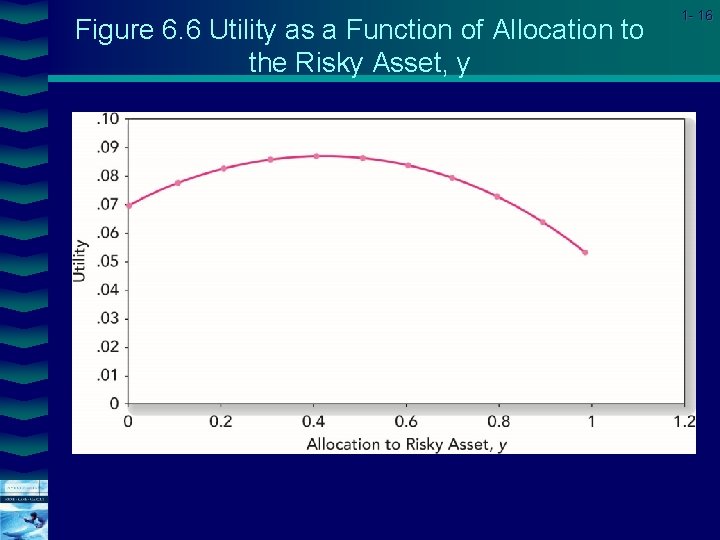
Figure 6. 6 Utility as a Function of Allocation to the Risky Asset, y Cover image 1 - 16

Figure 6. 7 Indifference Curves for U =. 05 and U =. 09 with A = 2 and A = 4 Cover image 1 - 17

Figure 6. 8 Finding the Optimal Complete Portfolio Using Indifference Curves Cover image 1 - 18

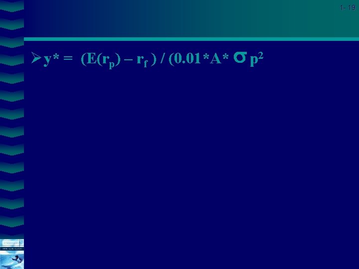
1 - 19 Ø y* = (E(rp) – rf ) / (0. 01*A* p 2 Cover image

Capital Market Line Ø Passive strategy: portfolio decision that avoids any direct or indirect security analysis Ø CML: investment opportunity set that generated by a passive strategy Cover image 1 - 20

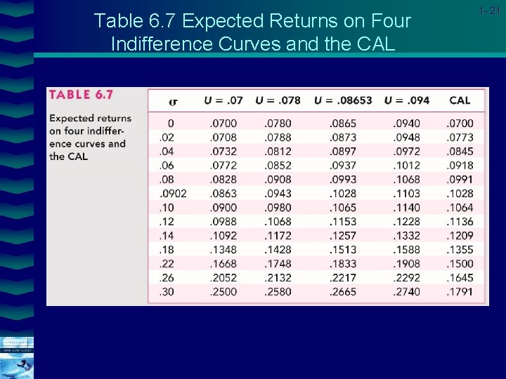
Table 6. 7 Expected Returns on Four Indifference Curves and the CAL Cover image 1 - 21

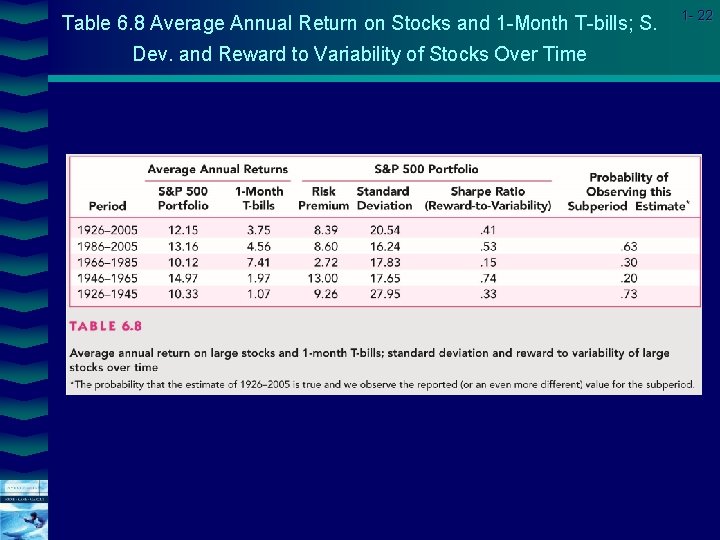
Table 6. 8 Average Annual Return on Stocks and 1 -Month T-bills; S. Dev. and Reward to Variability of Stocks Over Time Cover image 1 - 22