Risky Choices and Risk Aversion Chapter 18 Slides

Risky Choices and Risk Aversion Chapter 18 Slides by Pamela L. Hall Western Washington University © 2005, Southwestern

Introduction n A pyramid scheme is a fraudulent system of making money that requires an infinite stream of new investors for success § Recruits give money to recruiters and then enlist fresh recruits to § n give them money Such a scheme is called a pyramid scheme because it is the shape of a pyramid A similar scam is a Ponzi scheme § Named after Charles Ponzi who defrauded people in 1920 s • By getting people to invest in something for a guaranteed rate of return ¨ n Used money of later investors to pay off earlier ones The lesson? § Beware of any certain high rate of return • Nothing is certain but uncertainty 2

Introduction n General theory of agent choice under certainty cannot be employed for investigating optimal decisions with risky outcomes § Actual outcomes that occur in an uncertain world depend on their probability of occurring n n Based on both subjective and objective probabilities, we define risky alternatives (called states of nature) Given alternative states of nature, we define the Independence Axiom § Precludes states that will not happen from impacting household preferences n Given this Independence Axiom, we develop expected utility function as an interval measure of utility 3

Introduction n We define households’ risk preferences in terms of preferences § Risk-averse § Risk-seeking § Risk-neutral • Given a household’s risk preference, we develop concept of certainty equivalence along with its implications for insurance n n n We also develop concepts of actuarially fair insurance and asymmetric information associated with insurance Aim in this chapter is to introduce concepts of risk and uncertainty § Investigate impacts they have on agents’ decisions Expected utility is extensively used by applied economists as a tool for investigating this impact 4

Probability n A household’s decision regarding going to a movie this weekend has some probability associated with it § Even if household plans to go, something unexpected may occur and it would not go n Household will not go to movie if its opportunity cost of going rises to point where cost of going outweighs benefit § As household’s opportunity cost increases, probability of going to movie decreases n Probability is a measure of likelihood an outcome will occur § An outcome could be some level of income, amount or quality of a commodity, or a change in price n • If an outcome cannot happen, probability = 0 • If an outcome is certain to occur, probability = 1 In previous chapters, we assumed probabilities of all outcomes were either 0 or 1 5

Subjective Probability n Where a household has a perception that an event will occur § Household’s perception is based on • Conditions of current market prices • Its preferences • Its income n Any changes in these conditions will alter household’s perceptions § Households with different preferences will have different perceptions • Results in different subjective probabilities by individual households through time and across various households 6

Objective Probability n Frequency with which certain outcomes will occur § Objective probability of an outcome can be measured from past experiences n For example, if it is observed over some time interval that a household goes to movies once every 4 weeks § Probability of going to movie on any weekend is ¼ or 25% • An objective probability, measured by frequency of occurrence ¨ Depends on past household behavior 7

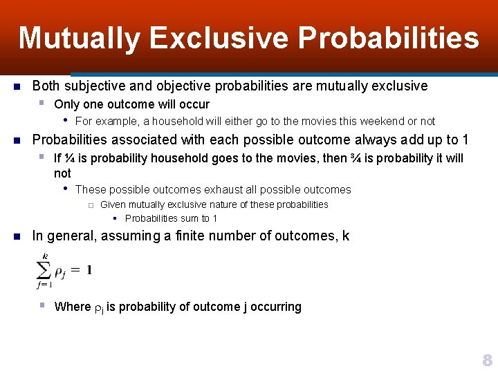
Mutually Exclusive Probabilities n Both subjective and objective probabilities are mutually exclusive § Only one outcome will occur n • For example, a household will either go to the movies this weekend or not Probabilities associated with each possible outcome always add up to 1 § If ¼ is probability household goes to the movies, then ¾ is probability it will not • These possible outcomes exhaust all possible outcomes ¨ n Given mutually exclusive nature of these probabilities § Probabilities sum to 1 In general, assuming a finite number of outcomes, k § Where j is probability of outcome j occurring 8

States of Nature n n In making future consumption plans, a household will consider probability of possible outcomes In determining these probabilities, household may use a combination of subjective and objective probabilities § Household is faced with choosing alternatives with uncertain § outcomes by means of known probabilities Each risky alternative is called a state of nature or lottery, N • Defined as a set of probabilities, summing to 1, with a probability assigned to each outcome n For example, state of nature associated with our household movie choice is (¼, ¾) § If probability of going to movies was ¾ and not going was ¼, state of nature would be reversed, (¾, ¼) 9

States of Nature n n n In general, a state of nature is a set of probabilities associated with all k outcomes Consistent with previous chapters, we assume households are rational when facing these states of nature with a preference relation Outcomes could be in any form § Including consumption bundles, money, or an opportunity to participate in another state of nature (called a compound lottery) n Fundamental difference between commodities and states of nature § Commodities can and generally are consumed jointly • Examples are driving and listening to radio § States of nature, by their definition of being mutually exclusive, cannot be consumed jointly • Either one state of nature exists or another ¨ For example, a household cannot have a 25% probability of going to the movies and a 75% probability of going to the movies at the same time • Idea of being unable to jointly consume two or more states of nature is a fundamental assumption of many theories dealing with choice under uncertainty ¨ Summarized by Independence Axiom 10

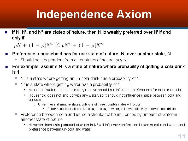
Independence Axiom n If N, N', and N" are states of nature, then N is weakly preferred over N' if and only if n Preference a household has for one state of nature, N, over another state, N' § Should be independent from other states of nature, say N" n For example, assume N is a state of nature where probability of getting a cola drink is 1 § N' is a state where getting an un-cola drink has a probability of 1 § N" is a state where getting water has a probability of 1 • Amount of water a household may receive should not influence preferences for cola or uncola • Household does not end up with any water, so it should not influence choice between cola and un-cola ¨ Under these alternative states, only one of three possible states will occur § Either household will receive cola, un-cola, or water, but it will not jointly receive these drinks § Preference between cola and un-cola should not be influenced by amount of water in another state of nature • However, increasing amount of water in N" will influence preference between cola and water and preference between un-cola and water 11

Expected Utility Function n n Suppose probability of a candidate for governor supporting environmental issues once elected (state of nature) varies by candidate Only one state of nature will actually occur § However, there is a probability associated with which state of nature will occur n Utility of environmentalists will vary depending on which candidate gets elected § Average (expected) utility from election is the sum of utilities for each candidate weighted by associated probability of being elected n Based on Independence Axiom, utility function for choice under uncertainty is additive for consumption in each possible state of nature § For all possible states of nature, utility from consumption in one state of nature is added to utility from consumption in another state • Called expected utility function or von Neumann–Morgenstern utility function) 12

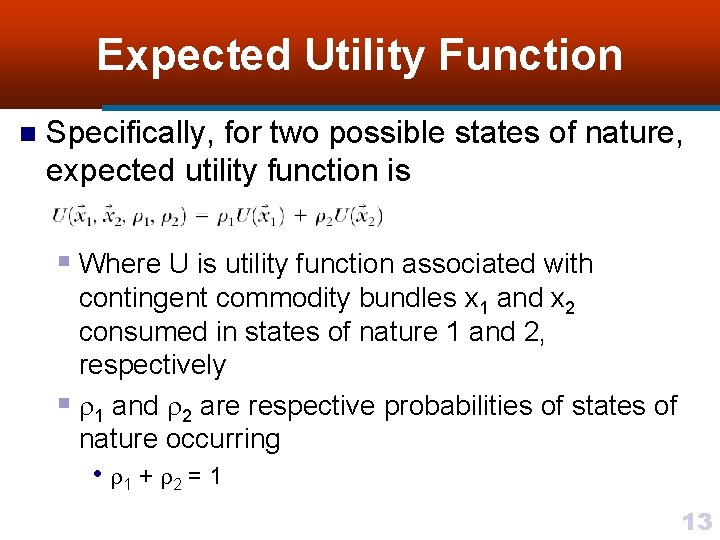
Expected Utility Function n Specifically, for two possible states of nature, expected utility function is § Where U is utility function associated with contingent commodity bundles x 1 and x 2 consumed in states of nature 1 and 2, respectively § 1 and 2 are respective probabilities of states of nature occurring • 1 + 2 = 1 13

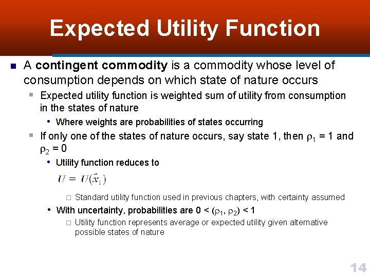
Expected Utility Function n A contingent commodity is a commodity whose level of consumption depends on which state of nature occurs § Expected utility function is weighted sum of utility from consumption in the states of nature • Where weights are probabilities of states occurring § If only one of the states of nature occurs, say state 1, then 1 = 1 and 2 = 0 • Utility function reduces to ¨ Standard utility function used in previous chapters, with certainty assumed • With uncertainty, probabilities are 0 < ( 1, 2) < 1 ¨ Utility function represents average or expected utility given alternative possible states of nature 14

Risk Preference n n Variability in outcomes of some state of nature when probability of each outcome is known is called risk Generally, statistical concept of variance is employed as a measure of risk § Variance is a measure of spread of a probability distribution measures variability in outcomes • The greater the variance and thus the variability in outcomes, the greater is the risk n For example, for a salaried employee the state of nature associated with receiving a fixed salary per month is risk free § It has no variability, no risk, and a variance of 0 § In contrast, an employee working on commission has some risk • The larger the variability in salary, possibly measured in terms of its variance, the greater the risk 15

Risk Preference n In general, unless compensated for risk exposure § Households appear to have an aversion to risk n In an effort to reduce this risk exposure, they will attempt to shift risk onto another agent § Purchasing insurance is a form of shifting risk • Its prevalence suggests risk aversion is common not only among households but also among firms 16

Risk Aversion n In a game of tossing a coin, if it is heads a household will receive $5 and if it is tails it must pay $5 § Expected value of game is ½(5) + ½(-5) = 0 • Called actuarially fair n Actuarially fair games § Games in which expected values are zero § Cost of playing a game is equivalent to game’s expected value n If instead payoff for heads is increased to $15, expected value would be § ½(15) + ½(-5) = 5 • A $5 cost of playing the game would reduce expected payoff to zero, which is actuarially fair n In terms of risk preferences, a household has risk-averse preferences if it refuses to play actuarially fair games § A risk-averse household would generally refuse to play these games • Unless there is some utility in actual process of playing and potential loss from playing is relatively small • It would prefer its current certain state to a risky state with a possible loss in happiness n Some individuals play actuarially unfair games § Expected value is negative • For some individuals who play slot machines or state lotteries, fun of playing and dreams of winning yield utility in excess of small cost of playing 17

Concave Utility Function n Risk-averse households would generally prefer a certain salary § Versus a variable salary based on sales with an expected value equivalent to certainty salary n A risk-averse household will not play actuarially fair games § For this household winning the game increases utility by a lesser degree than losing reduces it • Such a household prefers its current level of wealth over variance in wealth associated with an actuarially fair game ¨ Even though payoffs, in terms of resulting expected wealth, are the same 18

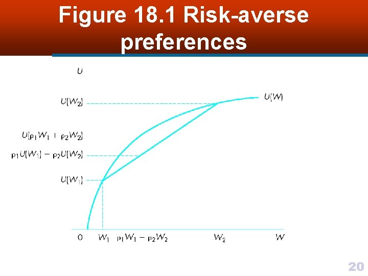
Concave Utility Function n Mathematically, for two possible states of nature, risk aversion may be stated as § U( 1 W 1 + 2 W 2) > 1 U(W 1) + 2 U(W 2) • Where W 1 and W 2 are levels of wealth resulting from possible outcomes 1 and 2, respectively § Level of utility associated with expected wealth, U( 1 W 1 + 2 W 2), is greater than state of nature resulting in expected utility of wealth, 1 U(W 1) + 2 U(W 2) n If outcomes were an employee’s salary, a risk-averse employee would prefer state of nature with certain salary resulting in U( 1 W 1 + 2 W 2) § Over uncertain salary with an expected utility level of 1 U(W 1) + 2 U(W 2) • Inequality is called Jensen’s inequality ¨ Defines concave function illustrated in Figure 18. 1 19

Figure 18. 1 Risk-averse preferences 20

Concave Utility Function n n A zero level of wealth corresponding with U = 0 results from a positive linear transformation of expected utility function Due to concave nature of utility function § Weighted average of wealth levels, W 1 and W 2, yield lower expected utility of wealth, 1 U(W 1) + 2 U(W 2), than utility of expected wealth, U( 1 W 1 + 2 W 2) • Weights are probability of wealth levels W 1 and W 2 occurring • 1 + 2 = 1 • 1 > 2 (in this case) n Risk aversion is equivalent to a concave expected utility function § Implies diminishing marginal utility of wealth • ∂2 U/∂W 2 < 0 ¨ As wealth increases, marginal utility of wealth declines 21

Risk Seeking n Some individuals may have risk-seeking preferences § Also called risk-loving preferences • Prefer a random distribution of wealth over its expected value § Gravitate toward occupations with more variable income streams • Examples are being self-employed, day-trading stocks, or working as a commodities trader n Some individuals are not only risk seeking in terms of their wealth, but also in life itself § Examples are race-car drivers, soldiers in special military forces, and criminals n Most individuals do not have such extreme risk-seeking preferences § However, at least for small potential losses in income, many households have some risk-seeking characteristics n • For example, many households engage in gambling Overall, households are generally risk averse when it comes to relatively large potential losses 22

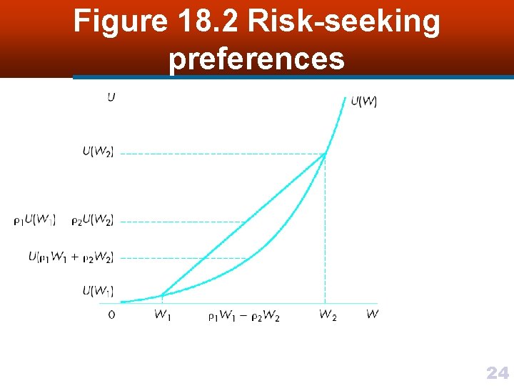
Risk Seeking n n n Mathematically, risk seeking reverses inequality for risk aversion For two possible states of nature, risk-seeking preferences are defined as § U( 1 W 1 + 2 W 2) < 1 U(W 1) + 2 U(W 2) As illustrated in Figure 18. 2, for risk-seeking preferences expected utility function is now convex § Weighted average of wealth levels, W 1 and W 2, yield a higher expected utility of wealth, 1 U(W 1) + 2 U(W 2), than utility of expected wealth, U( 1 W 1 + 2 W 2) • Risk seeking is equivalent to a convex expected utility function ¨ Implies increasing marginal utility of wealth, ∂2 U/∂W 2 > 0 § As wealth increases, marginal utility of wealth increases 23

Figure 18. 2 Risk-seeking preferences 24

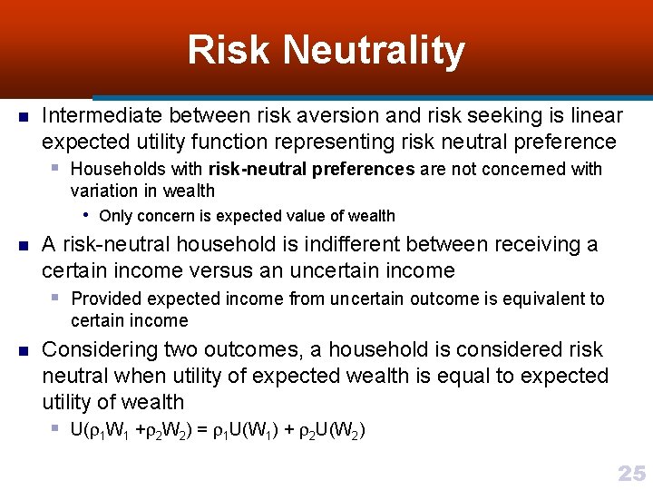
Risk Neutrality n Intermediate between risk aversion and risk seeking is linear expected utility function representing risk neutral preference § Households with risk-neutral preferences are not concerned with variation in wealth • Only concern is expected value of wealth n A risk-neutral household is indifferent between receiving a certain income versus an uncertain income § Provided expected income from uncertain outcome is equivalent to certain income n Considering two outcomes, a household is considered risk neutral when utility of expected wealth is equal to expected utility of wealth § U( 1 W 1 + 2 W 2) = 1 U(W 1) + 2 U(W 2) 25

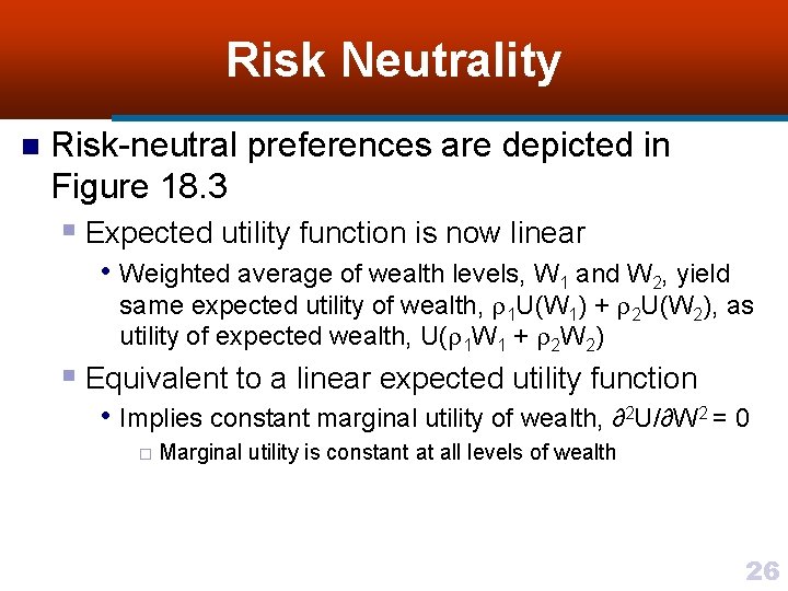
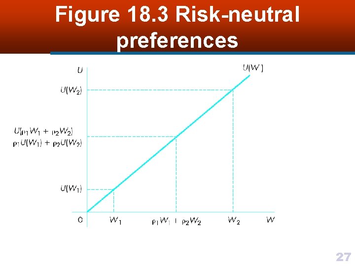
Risk Neutrality n Risk-neutral preferences are depicted in Figure 18. 3 § Expected utility function is now linear • Weighted average of wealth levels, W 1 and W 2, yield same expected utility of wealth, 1 U(W 1) + 2 U(W 2), as utility of expected wealth, U( 1 W 1 + 2 W 2) § Equivalent to a linear expected utility function • Implies constant marginal utility of wealth, ∂2 U/∂W 2 = 0 ¨ Marginal utility is constant at all levels of wealth 26

Figure 18. 3 Risk-neutral preferences 27

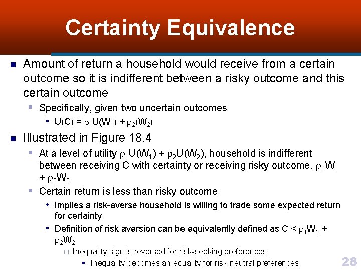
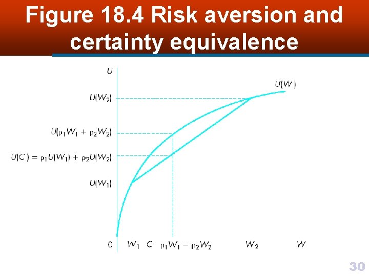
Certainty Equivalence n Amount of return a household would receive from a certain outcome so it is indifferent between a risky outcome and this certain outcome § Specifically, given two uncertain outcomes • U(C) = 1 U(W 1) + 2(W 2) n Illustrated in Figure 18. 4 § At a level of utility 1 U(W 1) + 2 U(W 2), household is indifferent § between receiving C with certainty or receiving risky outcome, 1 W 1 + 2 W 2 Certain return is less than risky outcome • Implies a risk-averse household is willing to trade some expected return • for certainty Definition of risk aversion can be equivalently defined as C < 1 W 1 + 2 W 2 ¨ Inequality sign is reversed for risk-seeking preferences § Inequality becomes an equality for risk-neutral preferences 28

Insurance n n Insurance companies have developed to where one can acquire an insurance policy against almost any risky outcome Certainty equivalence underlies functioning of insurance § Households are willing to pay to avoid risky outcomes • Maximum amount they are willing to pay is difference in expected wealth and certainty equivalence of wealth, ( 1 W 1 + 2 W 2) - C ¨ ¨ Paying more than this difference would result in a loss of utility They will be willing to pay less than this amount in the form of insurance premiums 29

Figure 18. 4 Risk aversion and certainty equivalence 30

Optimal Level of Insurance n n Can determine a household’s optimal level of insurance, A* § By assuming household has initial level of wealth, W, § Faces risk of sustaining a loss, D, with probability Household can reduce amount of loss by purchasing insurance, A, at a cost of p per-unit decrease in D (per-unit insurance premium) § Purchasing a level of insurance A will reduce loss from D to D - A § If outcome results in no loss occurring, household’s wealth is • W - p. A § If a loss occurs, household’s wealth level is • W – p. A – (D – A) ¨ Initial wealth minus total cost of insurance and net loss § Household’s expected wealth is § (1 - )(W – p. A) + [W – p. A – (D – A)] § Which reduces to W – p. A - (D – A) 31

Optimal Level of Insurance n n Although any expected utility function representing risk-averse preference can be employed, for simplicity assume following logarithmic expected utility function § U = (1 - ) ln(W – p. A) + ln[W – p. A – (D – A)] Can determine efficient level of insurance, A*, by maximizing this expected utility function § F. O. C. is • ∂U/∂A = -p(1 - )(W – p. A)-1 + p(1 - )[W – p. A – (D – A)]-1 = 0 32

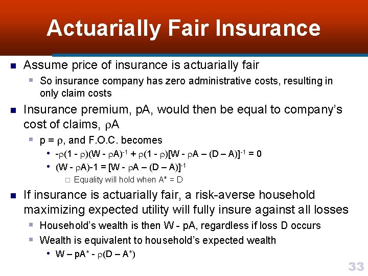
Actuarially Fair Insurance n Assume price of insurance is actuarially fair § So insurance company has zero administrative costs, resulting in only claim costs n Insurance premium, p. A, would then be equal to company’s cost of claims, A § p = , and F. O. C. becomes • - (1 - )(W - A)-1 + (1 - )[W - A – (D – A)]-1 = 0 • (W - A)-1 = [W - A – (D – A)]-1 ¨ n Equality will hold when A* = D If insurance is actuarially fair, a risk-averse household maximizing expected utility will fully insure against all losses § Household’s wealth is then W - p. A, regardless if loss D occurs § Wealth is equivalent to household’s expected wealth • W – p. A* - (D – A*) 33

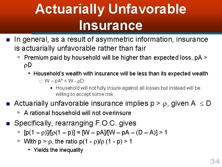
Actuarially Unfavorable Insurance n In general, as a result of asymmetric information, insurance is actuarially unfavorable rather than fair § Premium paid by household will be higher than expected loss, p. A > D • Household’s wealth with insurance will be less than its expected wealth ¨ n n W – p. A* < W - D § Household will not fully insure against all losses but instead will be willing to accept some risk Actuarially unfavorable insurance implies p > , given A D § A rational household will not overinsure Specifically, rearranging F. O. C. gives § [p(1 – )]/[ (1 – p)] = [W – p. A]/[W – p. A – (D – A)] > 1 § With p > , the ratio p(1 - )/ (1 - p) > 1 • Yields the inequality 34

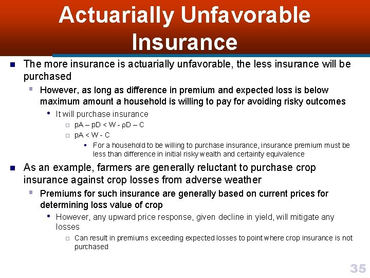
Actuarially Unfavorable Insurance n The more insurance is actuarially unfavorable, the less insurance will be purchased § However, as long as difference in premium and expected loss is below maximum amount a household is willing to pay for avoiding risky outcomes • It will purchase insurance ¨ ¨ n p. A – p. D < W - D – C p. A < W - C § For a household to be willing to purchase insurance, insurance premium must be less than difference in initial risky wealth and certainty equivalence As an example, farmers are generally reluctant to purchase crop insurance against crop losses from adverse weather § Premiums for such insurance are generally based on current prices for determining loss value of crop • However, any upward price response, given decline in yield, will mitigate any losses ¨ Can result in premiums exceeding expected losses to point where crop insurance is not purchased 35

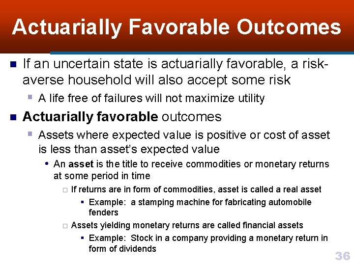
Actuarially Favorable Outcomes n n If an uncertain state is actuarially favorable, a riskaverse household will also accept some risk § A life free of failures will not maximize utility Actuarially favorable outcomes § Assets where expected value is positive or cost of asset is less than asset’s expected value • An asset is the title to receive commodities or monetary returns at some period in time ¨ ¨ If returns are in form of commodities, asset is called a real asset § Example: a stamping machine for fabricating automobile fenders Assets yielding monetary returns are called financial assets § Example: Stock in a company providing a monetary return in form of dividends 36

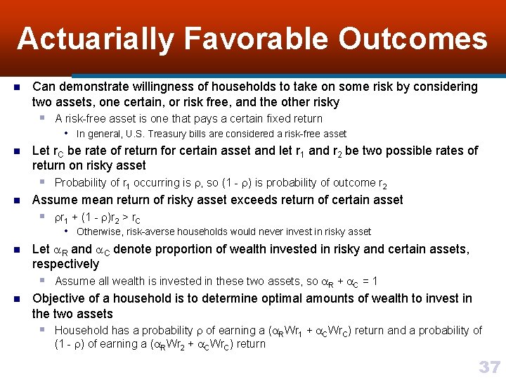
Actuarially Favorable Outcomes n Can demonstrate willingness of households to take on some risk by considering two assets, one certain, or risk free, and the other risky § A risk-free asset is one that pays a certain fixed return • In general, U. S. Treasury bills are considered a risk-free asset n Let r. C be rate of return for certain asset and let r 1 and r 2 be two possible rates of return on risky asset § Probability of r 1 occurring is , so (1 - ) is probability of outcome r 2 n Assume mean return of risky asset exceeds return of certain asset § r 1 + (1 - )r 2 > r. C • Otherwise, risk-averse households would never invest in risky asset n Let R and C denote proportion of wealth invested in risky and certain assets, respectively § Assume all wealth is invested in these two assets, so R + C = 1 n Objective of a household is to determine optimal amounts of wealth to invest in the two assets § Household has a probability of earning a ( RWr 1 + CWr. C) return and a probability of (1 - ) of earning a ( RWr 2 + CWr. C) return 37

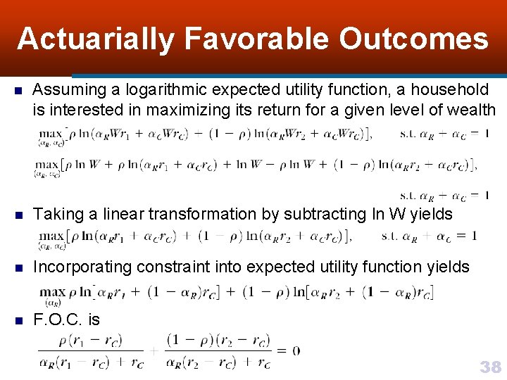
Actuarially Favorable Outcomes n Assuming a logarithmic expected utility function, a household is interested in maximizing its return for a given level of wealth n Taking a linear transformation by subtracting ln W yields n Incorporating constraint into expected utility function yields n F. O. C. is 38

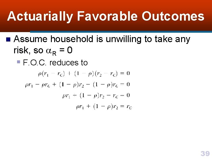
Actuarially Favorable Outcomes n Assume household is unwilling to take any risk, so R = 0 § F. O. C. reduces to 39

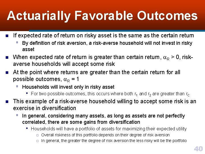
Actuarially Favorable Outcomes n If expected rate of return on risky asset is the same as the certain return § By definition of risk aversion, a risk-averse household will not invest in risky asset n n When expected rate of return is greater than certain return, R > 0, riskaverse households will accept some risk At the point where returns are greater than the certain return for all possible outcomes, R = 1 § Households will invest only in risky asset n • For two possible outcomes, this occurs where both r 1 and r 2 are greater than r. C This example of a risk-averse household willing to accept some risk is an exercise in diversification § In general, considering many assets, as long as assets are not perfectly correlated, there are some gains from diversification • Households will have a portfolio of assets for maximizing their expected utility ¨ ¨ Overall riskiness of this portfolio depends on their degree of risk aversion In general, the greater the degree of risk aversion the less risky will be the portfolio 40

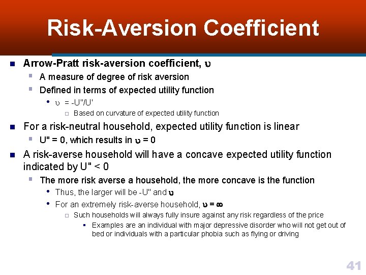
Risk-Aversion Coefficient n Arrow-Pratt risk-aversion coefficient, § A measure of degree of risk aversion § Defined in terms of expected utility function • = -U"/U' ¨ n Based on curvature of expected utility function For a risk-neutral household, expected utility function is linear § U" = 0, which results in = 0 n A risk-averse household will have a concave expected utility function indicated by U" < 0 § The more risk averse a household, the more concave is the function • Thus, the larger will be -U" and • For an extremely risk-averse household, = ¨ Such households will always fully insure against any risk regardless of the price § Examples are an individual with major depressive disorder who will not get out of bed or individuals with a particular phobia such as flying or driving 41

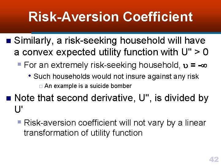
Risk-Aversion Coefficient n Similarly, a risk-seeking household will have a convex expected utility function with U" > 0 § For an extremely risk-seeking household, = - • Such households would not insure against any risk ¨ n An example is a suicide bomber Note that second derivative, U", is divided by U' § Risk-aversion coefficient will not vary by a linear transformation of utility function 42

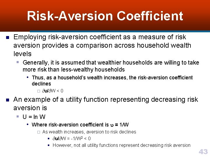
Risk-Aversion Coefficient n Employing risk-aversion coefficient as a measure of risk aversion provides a comparison across household wealth levels § Generally, it is assumed that wealthier households are willing to take more risk than less-wealthy households • Thus, as a household’s wealth increases, the risk-aversion coefficient declines ¨ n ∂ /∂W < 0 An example of a utility function representing decreasing risk aversion is § U = ln W • Where risk-aversion coefficient is = 1/W ¨ As wealth increases, aversion to risk declines § ∂ /∂W = -1/W 2 < 0 § However, not all utility functions represent decreasing risk aversion 43

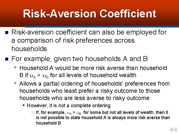
Risk-Aversion Coefficient n n Risk-aversion coefficient can also be employed for a comparison of risk preferences across households For example, given two households A and B § Household A would be more risk averse than household § B if A > B for all levels of household wealth Allows a partial ordering of households’ preferences from households who least prefer a risky outcome to those households who are less averse to risky outcome • However, it is not a complete ordering ¨ If, for example, A > B for some but not all levels of wealth, then it is not possible to state household A is always more risk averse than household B 44

State-Dependent Utility n A household may derive utility from not only the monetary returns § But also from states of nature that underline them n n • Called state-dependent utility Given this expected utility function for a household, we can determine utility-maximizing state of nature subject to a constraint on wealth Assume a household has a choice of two states of nature § For example, state 1 could be running its own business and § State 2 could be having a position in a large international firm n Associated with each state is a set (bundle) of contingent commodities § Each set is available only if the particular state occurs • By representing these commodity bundles in terms of monetary values (W 1 and • W 2) we can determine level of wealth required for obtaining each bundle Like all commodities, contingent commodities have an associated price ¨ This price is the cost of a particular uncertain state of nature occurring with certainty so that the associated contingent commodities may be received § Example: Political lobbyist’s expenditures on legislators to assure passage of some legislation 45

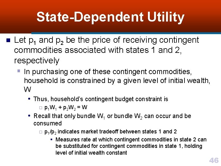
State-Dependent Utility n Let p 1 and p 2 be the price of receiving contingent commodities associated with states 1 and 2, respectively § In purchasing one of these contingent commodities, household is constrained by a given level of initial wealth, W • Thus, household’s contingent budget constraint is ¨ p 1 W 1 + p 2 W 2 = W • Recall that only bundle W 1 or bundle W 2 can occur and be consumed ¨ p 1/p 2 indicates market tradeoff between states 1 and 2 § Measures rate at which contingent commodities in state 2 can be substituted for contingent commodities in state 1, holding level of initial wealth constant 46

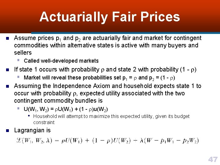
Actuarially Fair Prices n Assume prices p 1 and p 2 are actuarially fair and market for contingent commodities within alternative states is active with many buyers and sellers § Called well-developed markets n If state 1 occurs with probability and state 2 with probability (1 - ) § Market will reveal these probabilities set p 1 = and p 2 = (1 - ) n Assuming the Independence Axiom and household expects state 1 to occur with probability , expected utility associated with the two contingent commodity bundles is § U(W 1, W 2) = U(W 1) + (1 - )u(W 2) • Household will attempt to maximize this expected utility, given its budget constraint n Lagrangian is 47

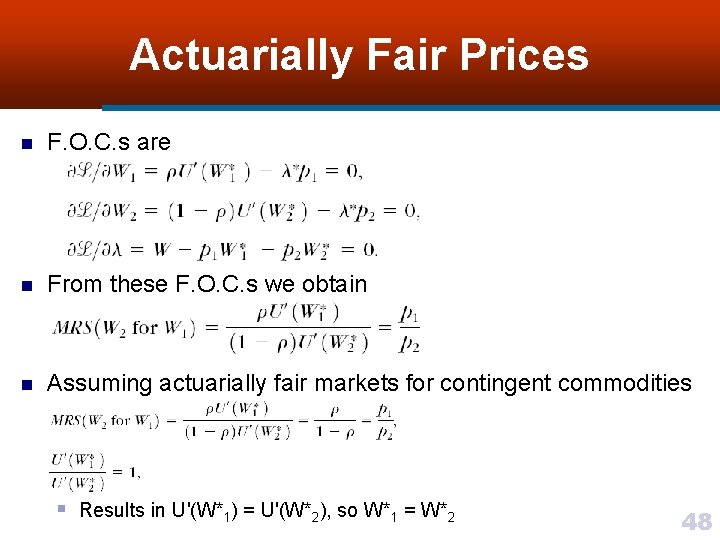
Actuarially Fair Prices n F. O. C. s are n From these F. O. C. s we obtain n Assuming actuarially fair markets for contingent commodities § Results in U'(W*1) = U'(W*2), so W*1 = W*2 48

Actuarially Fair Prices n Thus, a risk-averse household facing actuarially fair markets will be willing to pay for a state with certainty § Where final level of wealth is the same regardless of which state occurs • An example is market for insurance ¨ Where price for achieving a given state is the insurance premium and the contingent commodity is the contingent insurance claim 49

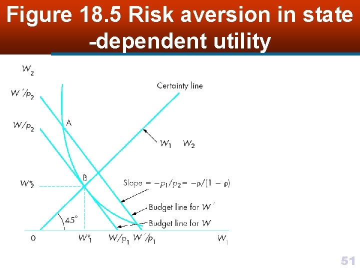
Actuarially Fair Prices n With actuarially fair insurance markets, risk-averse households will fully insure against possible losses § Will purchase insurance up to point where level of wealth is same regardless of whether state of nature involves a loss n • Illustrated in Figure 18. 5 Axes measure wealth for the two alternative states § Certainty line is a 45 line from origin n • Measures same level of wealth regardless of which state of nature occurs Indifference curves measure equivalent level of expected utility to certainty level associated with certainty line § Points not on certainty line represent utility levels associated with some uncertainty in which state of nature will occur n A household’s budget constraint is represented by budget line W § Every point on budget line represents actuarially fair probability of the two states of nature occurring 50

Figure 18. 5 Risk aversion in state -dependent utility 51

Actuarially Fair Prices n A risk-averse household is unwilling to play an actuarially fair game § Movements off certainty line on budget line will result in lower levels of utility • For a risk-averse household to be willing to accept some risk, they must be compensated in the form of additional wealth ¨ n A risk-averse household has indifference curves that are convex to origin Point A is unobtainable with initial wealth W § However, at point A § Household can maintain same level of utility, but requiring less initial wealth • By moving down along indifference curve ¨ Decrease in required initial wealth continues until point B is reached on certainty line § Where wealth levels of the states are equal 52

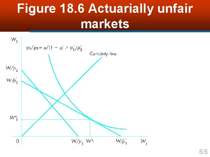
Actuarially Unfair Prices n If market is actuarially unfair, a risk-averse household may choose to accept some risk § For example, consider an unfair price ratio of p 1/p 2 < /(1 - ) § From F. O. C. s for expected utility maximization § Assuming actuarially unfair condition p 1/p 2 < /(1 - ) • Results in U'(W*1) < U'(W*2) ¨ So, assuming diminishing marginal utility of income, W*1 > W*2 53

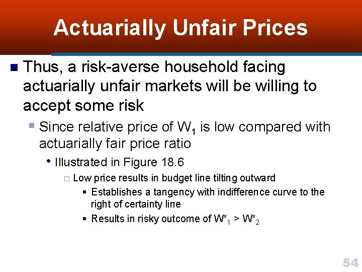
Actuarially Unfair Prices n Thus, a risk-averse household facing actuarially unfair markets will be willing to accept some risk § Since relative price of W 1 is low compared with actuarially fair price ratio • Illustrated in Figure 18. 6 ¨ Low price results in budget line tilting outward § Establishes a tangency with indifference curve to the right of certainty line § Results in risky outcome of W*1 > W*2 54

Figure 18. 6 Actuarially unfair markets 55

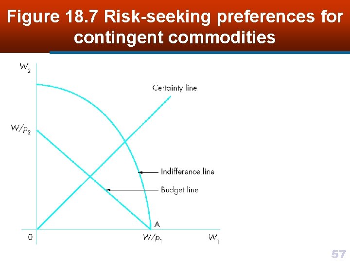
Risk Seeking n A risky outcome will also result if a household is risk seeking § Illustrated in Figure 18. 7 n Risk-seeking household’s indifference curves are concave from origin § Implies expected value for a certain outcome must be higher than any risky outcome before household would be indifferent between outcomes • Results in a corner solution, point A ¨ Household prefers outcome with greater risk 56

Figure 18. 7 Risk-seeking preferences for contingent commodities 57