Introductory Macroeconomics Semester4 CC8 Theory of intertemporal choice

Introductory Macroeconomics Semester-4, CC-8 Theory of intertemporal choice- Irving Fisher Prepared by Abanti Goswami Ref. (1) G. Mankiw (2) Ambar Ghosh & Chandana Ghosh

Irving Fisher and Intertemporal Choice � The economist Irving Fisher developed the model with which economists analyze how rational, forward-looking consumers make intertemporal choices— that is, choices involving different periods of time. � Fisher’s model analyses the constraints the consumers face and the preferences they have. � The model discusses how these constraints and preferences together determine the consumers’ choices about consumption and saving.

� The Keynesian consumption function relates current consumption to current income. But this relationship, however, is incomplete at best. � When people decide how much to consume and how much to save, they make a tradeoff between the present and the future. � Households must look ahead to the income they expect to receive in the future and to the consumption of goods and services they hope to be able to afford.

� The intertemporal budget constraint shows that people consume less than they desire as their consumption is constrained by their income. � When they are deciding how much to consume today versus how much to save for the future, they face an intertemporal budget constraint, which measures the total resources available for consumption today and in the future. � Our first step in developing Fisher’s model is to examine this constraint in some detail.

�. We examine the decision facing a consumer who lives for two periods. Period one represents the consumer’s youth, and period two represents the consumer’s old age. � The consumer earns income Y 1 and consumes C 1 in period one, and earns income Y 2 and consumes C 2 in period two. (All variables are real —that is, adjusted for inflation. ) � Because the consumer has the opportunity to borrow and save, consumption in any single period can be either greater or less than income in that period. � Consider how the consumer’s income in the two periods constrains consumption in the two periods. In the first period, saving equals income minus consumption. That is, S = Y 1 − C 1, where S is saving.

� In the second period, consumption equals the accumulated saving, including the interest earned on that saving, plus second-period income. � C 2 = (1 + r)S + Y 2, where r is the real interest rate. Because there is no third period, the consumer does not save in the second period. � Note that the variable S can represent either saving or borrowing and that these equations hold in both cases. If first-period consumption is less than first-period income, the consumer is saving, and S is greater than zero. If first-period consumption exceeds first-period income, the consumer is borrowing, and S is less than zero. � For simplicity, we assume that the interest rate for borrowing is the same as the interest rate for saving.

� To derive the consumer’s budget constraint, combine the two preceding equations. � Substitute the first equation for S into the second equation to obtain C 2 = (1 + r)(Y 1 − C 1) + Y 2. � To make the equation easier to interpret, we must rearrange terms. To place all the consumption terms together, bring (1+r)C 1 from the right-hand side to the left-hand side of the equation to obtain (1 + r)C 1 + C 2 = (1 + r)Y 1 + Y 2. � Now divide both sides by 1 + r to obtain C 1 +C 2/1+r = Y 1 +Y 2/1+r.

� This equation relates consumption in the two periods to income in the two periods. It is the standard way of expressing the consumer’s intertemporal budget constraint. � If the interest rate is zero, the budget constraint shows that total consumption in the two periods equals total income in the two periods. � If interest rate is greater than zero, future consumption and future income are discounted by a factor 1 + r. This discounting arises from the interest earned on savings. The consumer earns interest on current income that is saved, future income is worth less than current income. Similarly, because future consumption is paid for out of savings that have earned interest, future consumption costs less than current consumption.

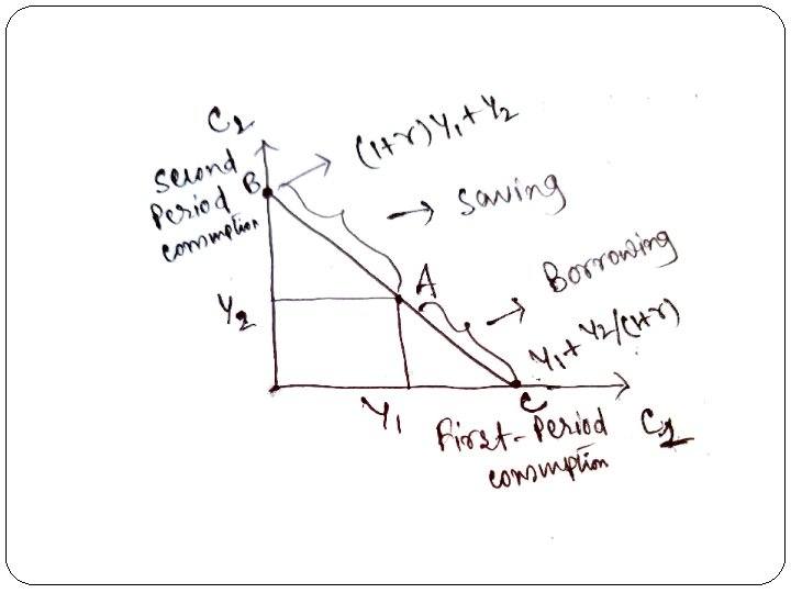
� The factor 1/ (1 + r) is the price of second-period consumption measured in terms of first-period consumption. It is the amount of first -period consumption that the consumer must forgo to obtain 1 unit of second-period consumption. � The following figure graphs the consumer’s budget constraint. Three points are marked on this figure.

� At point A, the consumer consumes exactly his income in each period (C 1 = Y 1 and C 2 = Y 2), so there is neither saving nor borrowing between the two periods. � At point B, the consumer consumes nothing in the first period (C 1 = 0) and saves all income, so second-period consumption C 2 is (1 + r) Y 1 + Y 2. � At point C, the consumer plans to consume nothing in the second period (C 2 = 0) and borrows as much as possible against second-period income, so first-period consumption C 1 is Y 1 + Y 2/ (1 + r). � These are only three of the many combinations of first- and second- period consumption that the consumer can afford: all the points on the line from B to C are available to the consumer.

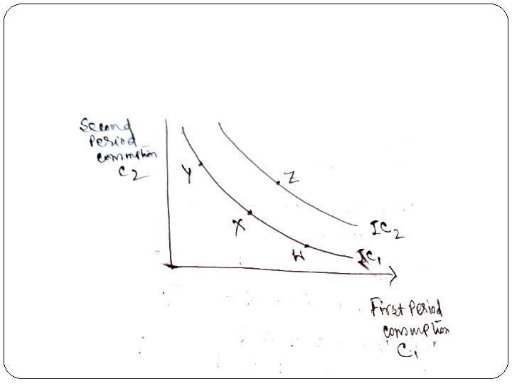
� The consumer’s preferences regarding consumption in the two periods can be represented by indifference curves. An indifference curve shows the combinations of first-period and second-period consumption that make the consumer equally happy. � Above figure shows two of the consumer’s indifference curves. The consumer is indifferent among combinations W, X, and Y, because they are all on the same curve. � If the consumer’s first-period consumption is reduced, say from point W to point X, second-period consumption must increase to keep him equally happy. If first-period consumption is reduced again, from point X to point Y, the amount of extra second-period consumption he requires for compensation is greater.

� The slope at any point on the indifference curve shows how much second period consumption the consumer requires in order to be compensated for a 1 -unit reduction in first-period consumption. � This slope is the marginal rate of substitution between first-period consumption and second-period consumption. It tells us the rate at which the consumer is willing to substitute second-period consumption for first-period consumption. � the indifference curves in Figure are not straight lines; as a result, the marginal rate of substitution depends on the levels of consumption in the two periods.

� When first-period consumption is high and second-period consumption is low, as at point W, the marginal rate of substitution is low and the consumer requires only a little extra second-period consumption to give up. � When first-period consumption is low and second-period consumption is high, as at point Y, the marginal rate of substitution is high: the consumer requires much additional second-period consumption to give up 1 unit of first-period consumption. The consumer is equally happy at all points on a given indifference curve. � He prefers more consumption to less, he prefers higher indifference curves to lower ones.

� The consumer prefers any of the points on curve IC 2 to any of the points on curve IC 1. � The set of indifference curves gives a complete ranking of the consumer’s preferences. It tells us that the consumer prefers point Z to point W, but that should be obvious because point Z has more consumption in both periods. � Compare point Z and point Y: point Z has more consumption in period one and less in period two. � Because Z is on a higher indifference curve than Y, we know that the consumer prefers point Z to point Y. Hence, we can use the set of indifference curves to rank any combinations of first-period and secondperiod consumption.

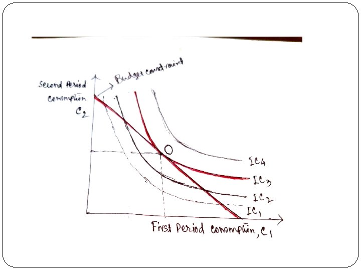
� Having discussed the consumer’s budget constraint and preferences, we can consider the decision about how much to consume in each period of time. � The consumer would like to end up with the best possible combination of consumption in the two periods—that is, on the highest possible indifference curve. � But the budget constraint requires that the consumer also end up on or below the budget line, because the budget line measures the total resources available to him. � The following figure shows the fact.

� The highest indifference curve that the consumer can obtain without violating the budget constraint is the indifference curve that just touches the budget line, which is curve IC 3 in the figure. � The point at which the curve and line touch—point O, for “optimum” —is the best combination of consumption in the two periods that the consumer can afford. � At the optimum, the slope of the indifference curve equals the slope of the budget line. The indifference curve is tangent to the budget line. The slope of the indifference curve is the marginal rate of substitution MRS, and the slope of the budget line is 1 +r. � We conclude that. The consumer chooses consumption in the two periods such that the marginal rate of substitution equals 1+r.