Introduction to Software Testing Chapter 4 Input Space

Introduction to Software Testing Chapter 4 Input Space Partition Testing Paul Ammann & Jeff Offutt http: //www. cs. gmu. edu/~offutt/soft waretest/

Ch. 4 : Input Space Coverage Four Structures for Modeling Software Graphs Logic Input Space Syntax Applied to Source FSMs Specs Source Applied to DNF Source Specs Design Introduction to Software Testing (Ch 4) Models Integ Use cases © Ammann & Offutt Input 2

Input Domains • The input domain to a program contains all the possible inputs to that program • For even small programs, the input domain is so large that it might as well be infinite • Testing is fundamentally about choosing finite sets of values from the input domain • Input parameters define the scope of the input domain – – Parameters to a method Data read from a file Global variables User level inputs • Domain for each input parameter is partitioned into regions • At least one value is chosen from each region Introduction to Software Testing (Ch 4) © Ammann & Offutt 3

Benefits of ISP • Can be equally applied at several levels of testing – Unit – Integration – System • Relatively easy to apply with no automation • Easy to adjust the procedure to get more or fewer tests • No implementation knowledge is needed – just the input space Introduction to Software Testing (Ch 4) © Ammann & Offutt 4

Partitioning Domains • • Domain D Partition scheme (characteristic) q of D The partition q defines a set of blocks, Bq = b 1 , b 2 , … b. Q The partition must satisfy two properties : 1. blocks must be pairwise disjoint (no overlap) 2. together the blocks cover the domain D (complete) b 1 b 2 bi bj = , i j, bi, bj Bq b 3 Introduction to Software Testing (Ch 4) b=D b Bq © Ammann & Offutt 5

Using Partitions – Assumptions • Choose a value from each partition • Each value is assumed to be equally useful for testing • Application to testing – Find characteristics in the inputs : parameters, semantic descriptions, … – Partition each characteristic – Choose tests by combining values from characteristics • Example Characteristics – – Input X is null Order of the input file F (sorted, inverse sorted, arbitrary, …) Min separation of two aircraft Input device (DVD, CD, VCR, computer, …) Introduction to Software Testing (Ch 4) © Ammann & Offutt 6

Choosing Partitions • Choosing (or defining) partitions seems easy, but it is easy to get wrong • Consider the “order of file F” b 1 = sorted in ascending order b 2 = sorted in descending order b 3 = arbitrary order but … something’s fishy … What if the file is of length 1? Problem: The file will be in all three blocks, thus disjointness is not satisfied Solution: Each characteristic should address just one property 1. C 1: File F sorted ascending: C 1. b 1 = true, 2. C 2: File F sorted descending: C 2. b 1 = true, Introduction to Software Testing (Ch 4) © Ammann & Offutt C 1. b 2 = false C 2. b 2 = false 7

Properties of Partitions • If the partitions are not complete or disjoint, that means the partitions have not been considered carefully enough • They should be reviewed carefully, like any design attempt • Different alternatives should be considered • We model the input domain in five steps … – Steps 1 and 2 move us from the implementation abstraction level to the design abstraction level (from chapter 2) – Steps 3 & 4 are entirely at the design abstraction level – Step 5 brings us back down to the implementation abstraction level Introduction to Software Testing (Ch 4) © Ammann & Offutt 8

Modeling the Input Domain • Step 1 : Identify testable functions – Individual methods have one testable function – In a class, each method often has the same characteristics – Programs have more complicated characteristics—modeling documents such as UML use cases can be used to design characteristics – Systems of integrated hardware and software components can use devices, operating systems, hardware platforms, browsers, etc. • Step 2 : Find all the parameters – Often fairly straightforward, even mechanical – Important to be complete – Methods : Parameters and state (non-local) variables used – Components : Parameters to methods and state variables – System : All inputs, including files and databases Introduction to Software Testing (Ch 4) © Ammann & Offutt 9

Modeling the Input Domain (cont. ) • Step 3 : Model the input domain (IDM) – The domain is scoped by the parameters – The structure is defined in terms of characteristics – Each characteristic is partitioned into sets of blocks – Each block represents a set of values – This is the most creative design step in applying ISP • Step 4 : Apply a test criterion to choose combinations of values – A test input has a value for each parameter – One block for each characteristic – Choosing all combinations is usually infeasible – Coverage criteria allow subsets to be chosen • Step 5 : Refine combinations of blocks into test inputs – Choose appropriate values from each block Introduction to Software Testing (Ch 4) © Ammann & Offutt 10

Two Approaches to Input Domain Modeling (IDM) 1. Interface-based approach – Develops characteristics directly from individual input parameters – Simplest application – Can be partially automated in some situations 2. Functionality-based approach – Develops characteristics from a behavioral view of the program under test – Harder to develop—requires more design effort – May result in better tests, or fewer tests that are as effective Introduction to Software Testing (Ch 4) © Ammann & Offutt 11

1. Interface-Based Approach • Mechanically consider each parameter in isolation • This is an easy modeling technique and relies mostly on syntax • Some domain and semantic information won’t be used – Could lead to an incomplete IDM • Ignores relationships among parameters Introduction to Software Testing (Ch 4) © Ammann & Offutt 12

1. Interface-Based Example • Consider method triang() from class Triangle. Type on the book website : – http: //www. cs. gmu. edu/~offutt/softwaretest/edition 2/java/Triangle. java – http: //www. cs. gmu. edu/~offutt/softwaretest/edition 2/java/Triangle. Type. java public enum Triangle { Scalene, Isosceles, Equilateral, Invalid } public static Triangle triang (int Side 1, int Side 2, int Side 3) // Side 1, Side 2, and Side 3 represent the lengths of the sides of a triangle // Returns the appropriate enum value The IDM for each parameter is identical Reasonable characteristic : Relation of side with zero Introduction to Software Testing, Edition 2 (Ch 6) © Ammann & Offutt 13

2. Functionality-Based Approach • Identify characteristics that correspond to the intended functionality • Requires more design effort from tester • Can incorporate domain and semantic knowledge • Can use relationships among parameters • Modeling can be based on requirements, not implementation • The same parameter may appear in multiple characteristics, so it’s harder to translate values to test cases Introduction to Software Testing (Ch 4) © Ammann & Offutt 14

2. Functionality-Based Example • Again, consider method triang() from class Triangle. Type : The three parameters represent a triangle The IDM can combine all parameters Reasonable characteristic : Type of triangle Introduction to Software Testing, Edition 2 (Ch 6) © Ammann & Offutt 15

Steps 1 & 2 – Identifying Functionalities, Parameters and Characteristics • • A creative engineering step More characteristics means more tests Interface-based : Translate parameters to characteristics Candidates for characteristics : – Pre- and Post-conditions – Relationships among variables – Relationship of variables with special values (zero, null, blank, …) • Should not use program source – Characteristics should be based on the input domain – Program source should be used with graph or logic criteria • Better to have more characteristics with few blocks – Fewer mistakes and fewer tests Introduction to Software Testing (Ch 4) © Ammann & Offutt 16

Steps 1 & 2 : Interface vs. Functionality-Based public boolean find. Element (List list, Object element) // Effects: if list or element is null throw Null. Pointer. Exception // else return true if element is in the list, false otherwise Interface-Based Approach Two parameters : list, element Characteristics : C 1: list is null (b 1 = true, b 2 = false) C 2: list is empty (b 1 = true, b 2 = false) Functionality-Based Approach Two parameters : list, element Characteristics : C 1: number of occurrences of element in list (b 1 = 0, b 2 = 1, b 3 = >1) C 2: element occurs first in list (b 1 = true, b 2 = false) C 3: element occurs last in list (b 1 = true, b 2 = false) Introduction to Software Testing (Ch 4) © Ammann & Offutt 17

Step 3 : Modeling the Input Domain • Partitioning characteristics into blocks and values is a very creative engineering step • More blocks means more tests • The partitioning often flows directly from the definition of characteristics and both steps are sometimes done together – Should evaluate them separately – sometimes fewer characteristics can be used with more blocks and vice versa • Strategies for identifying values : – – – Include valid, invalid, and special values Sub-partition some blocks Explore boundaries of domains Include values that represent “normal use” Try to balance the number of blocks in each characteristic Check for completeness and disjointness Introduction to Software Testing (Ch 4) © Ammann & Offutt 18

Interface-Based IDM – Tri. Typ • Tri. Typ, from Chapter 3, had one testable function and three integer inputs First Characterization of Tri. Typ’s Inputs Characteristic b 1 b 2 b 3 q 1 = “Relation of Side 1 to 0” greater than 0 equal to 0 less than 0 q 2 = “Relation of Side 2 to 0” greater than 0 equal to 0 less than 0 q 3 = “Relation of Side 3 to 0” greater than 0 equal to 0 less than 0 • A maximum of 3*3*3 = 27 possible tests • Some triangles are valid, some are invalid • Refining the characterization can lead to more tests … Introduction to Software Testing (Ch 4) © Ammann & Offutt 19

Interface-Based IDM – Tri. Typ (cont. ) Second Characterization of Tri. Typ’s Inputs Characteristic b 1 b 2 b 3 b 4 q 1 = “Refinement of q 1” greater than 1 equal to 0 less than 0 q 2 = “Refinement of q 2” greater than 1 equal to 0 less than 0 q 3 = “Refinement of q 3” greater than 1 equal to 0 less than 0 • A maximum of 4*4*4 = 64 possible tests • This is only complete because the inputs are integers (0. . 1) Possible values for partition q 1 Characteristic b 1 b 2 b 3 Side 1 Introduction to Software Testing (Ch 4) 52 1 0 Test boundary conditions b 4 -5 -1 20

Functionality-Based IDM – Tri. Typ • First two characterizations are based on syntax: parameters and their type • A semantic level characterization could use the fact that the three integers (parameters) represent a triangle Geometric Characterization of Tri. Typ’s Inputs Characteristic b 1 b 2 b 3 b 4 q 1 = “Geometric Classification” scalene isosceles equilateral invalid • Oops … something’s fishy … equilateral is also isosceles ! • We need to refine the example to make characteristics valid Correct Geometric Characterization of Tri. Typ’s Inputs Characteristic b 1 b 2 b 3 b 4 q 1 = “Geometric Classification” scalene isosceles, not equilateral Introduction to Software Testing (Ch 4) © Ammann & Offutt invalid 21

Functionality-Based IDM – Tri. Typ (cont. ) • Values for this partitioning can be chosen as Possible values for geometric partition q 1 Characteristic b 1 b 2 b 3 Triangle Introduction to Software Testing (Ch 4) (4, 5, 6) (3, 3, 4) © Ammann & Offutt (3, 3, 3) b 4 (3, 4, 8) 22

Functionality-Based IDM – Tri. Typ (cont. ) • A different approach would be to break the geometric characterization into four separate characteristics Four Characteristics for Tri. Typ Characteristic b 1 b 2 q 1 = “Scalene” True False q 2 = “Isosceles” True False q 3 = “Equilateral” True False q 4 = “Valid” True False • Use constraints to ensure that – Equilateral = True implies Isosceles = True – Valid = False implies Scalene = Isosceles = Equilateral = False Introduction to Software Testing (Ch 4) © Ammann & Offutt 23

Using More than One IDM • Some programs may have dozens or even hundreds of parameters • Create several small IDMs – A divide-and-conquer approach • Different parts of the software can be tested with different amounts of rigor (consistency, accuracy, care, etc. ) – For example, some IDMs may include a lot of invalid values • It is okay if the different IDMs overlap – The same variable may appear in more than one IDM Introduction to Software Testing (Ch 4) © Ammann & Offutt 24

The Test Selection Problem • The input domain of a program consists of all possible inputs that could be taken by the program. • Ideally, the test selection problem is to select a subset T of the input domain such that the execution of T will reveal all errors. • In practice, the test selection problem is to select a subset of T within budget such that it reveals as many errors as possible. Introduction to Software Testing (Ch 4) © Ammann & Offutt 25

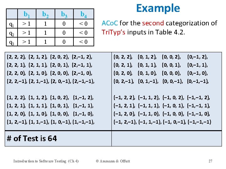
Step 4 – Choosing Combinations of Values • Once characteristics and partitions are defined, the next step is to choose test values • We use criteria – to choose effective subsets • The most obvious criterion is to choose all combinations All Combinations Coverage (ACo. C) : All combinations of blocks from all characteristics must be used. • Number of tests is the product of the number of blocks in each Q characteristic : (B ) i=1 i • The second characterization of Tri. Typ results in 4*4*4 = 64 tests – too many ? Introduction to Software Testing (Ch 4) © Ammann & Offutt 26

ISP Criteria – Each Choice • 64 tests for Tri. Typ is almost certainly way too many • One criterion comes from the idea that we should try at least one value from each block Each Choice Coverage (ECC) : One value from each block for each characteristic must be used in at least one test case. • Number of tests is at least the number of blocks in the largest Q characteristic (B ) i=1 i Max q 1 q 2 q 3 b 1 b 2 b 3 b 4 >1 >1 >1 1 0 0 0 <0 <0 <0 Introduction to Software Testing (Ch 4) For Tri. Typ: 2, 2, 2 1, 1, 1 0, 0, 0 -1, -1 © Ammann & Offutt 28

ISP Criteria – Pair-Wise • Each Choice (ECC) yields few tests – cheap but perhaps ineffective • Another approach asks values to be combined with other values Pair-Wise Coverage (PWC) : A value from each block for each characteristic must be combined with a value from every block for each other characteristic. • Number of tests is at least the product of two largest Q Q characteristics (Bi) (Bj) j=1, j!=i i=1 (Max q 1 q 2 q 3 ) * (Max b 1 b 2 b 3 b 4 For Tri. Typ: >1 >1 >1 1 0 0 0 <0 <0 <0 2, 2, 2 2, 1, 1 1, 2, 1 0, 2, 0 -1, 2, -1 1, 1, 0, -1 0, 1, -1 0, 0, 2 -1, 1, 2 -1, 0, 1 Introduction to Software Testing (Ch 4) © Ammann & Offutt 2, 0, 0 ) 2, -1 1, -1, 2 0, -1, 1 -1, 0 29

Example • Assume that we have three partitions, each is divided into blocks b 1 b 2 C 1 A B ACo. C (A, 1, x) (A, 1, y) (A, 2, x) (A, 2, y) (A, 3, x) (A, 3, y) • (B, 1, x) (B, 1, y) (B, 2, x) (B, 2, y) (B, 3, x) (B, 3, y) # of Tests is 2 * 3 * 2 = 12 b 1 b 2 b 3 C 2 1 2 3 C 3 x y PWC ECC can be satisfied in many ways. i. e. (A, 1, x) (B, 2, y) (A, 3, x) • # of Tests is 3 Introduction to Software Testing (Ch 4) b 1 b 2 • All Pairs (A, 1) (B, 1) (A, 2) (B, 2) (A, 3) (B, 3) (A, x) (B, x) (A, y) (B, y) But: (1, x) PWC allows the same test case to cover more than (1, y) one unique pair of values (2, x) (A, 1, x) (B, 1, y) (2, y) (A, 2, x) (B, 2, y) (3, x) (A, 3, x) (B, 3, y) (A, _, y) (B, _, x) • # of all pairs • # of Tests is (2 * 3) + 6 (2 * 2) + (3 * 2) = 16 © Ammann & Offutt 30

ISP Criteria –T-Wise • A natural extension is to require combinations of T values instead of 2 T-Wise Coverage (TWC) : A value from each block for each group of T characteristics must be combined. • Number of tests is at least the product of T largest characteristics • If all characteristics are the same size, the formula is (Max Q t (B ) i=1 i ) • If T is the number of characteristics Q, then all combinations • That is … Q-wise = ACo. C • T-Wise is expensive and benefits are not clear Introduction to Software Testing (Ch 4) © Ammann & Offutt 31

ISP Criteria – Base Choice /1 • Both PWC and TWC combine values “blindly” without regard for which values are being combined • Testers sometimes recognize that certain values are more important than others • This important value is called Base Choice – It can be obtained by asking what is the most “important” block for each partition • Simply, Base Choice strengthens ECC by utilizing information about the domain (domain knowledge) • The Base Choice can be – – the simplest, the smallest, the first in some ordering, or the most likely from an end-user point of view, … etc. Introduction to Software Testing (Ch 4) © Ammann & Offutt 32

ISP Criteria – Base Choice /2 Base Choice Coverage (BCC) : A base choice block is chosen for each characteristic, and a base test is formed by using the base choice for each characteristic. Subsequent tests are chosen by holding all but one base choice constant and using each non-base choice in each other characteristic. • Number of tests is one base test + one test for each other block Q 1 + i=1 (Bi -1 ) Our Base Choice Block q 1 q 2 q 3 b 1 b 2 b 3 b 4 >1 >1 >1 1 0 0 0 <0 <0 <0 Introduction to Software Testing (Ch 4) For Tri. Typ: Base is 2, 2, 2 (>1 is our BC) 2, 2, 1 2, 2, 0 2, 2, -1 © Ammann & Offutt 2, 1, 2 2, 0, 2 2, -1, 2, 2 0, 2, 2 -1, 2, 2 33

ISP Criteria – Multiple Base Choice • Testers sometimes have more than one logical base choice Multiple Base Choice Coverage (MBCC) : One or more base choice blocks are chosen for each characteristic, and base tests are formed by using each base choice for each characteristic. Subsequent tests are chosen by holding all but one base choice constant for each base test and using each non-base choices in each other characteristic. • If there are M base tests and mi Base Choices for each Q characteristic: M + i=1 (M * (Bi - mi )) For Tri. Typ: Base (two base choices: >1 and 1) Our two Base Choice Block q 1 q 2 q 3 b 1 b 2 b 3 b 4 >1 >1 >1 1 0 0 0 <0 <0 <0 Introduction to Software Testing (Ch 4) 2, 2, 2 : 2, 2, 0 2, 2, -1 1, 1, 1 : 1, 1, 0 1, 1, -1 © Ammann & Offutt 2, 0, 2 2, -1, 2 1, 0, 1 1, -1, 1 0, 2, 2 -1, 2, 2 0, 1, 1 -1, 1, 1 34

ISP Coverage Criteria Subsumption All Combinations Coverage ACo. C T-Wise Coverage TWC Multiple Base Choice Coverage MBCC Pair-Wise Coverage PWC Base Choice Coverage BCC Each Choice Coverage ECC Introduction to Software Testing (Ch 4) © Ammann & Offutt 35

Constraints Among Characteristics • Some combinations of blocks are infeasible – “less than zero” and “scalene” … not possible at the same time • These are represented as constraints among blocks • Two general types of constraints – A block from one characteristic cannot be combined with a specific block from another – A block from one characteristic can ONLY BE combined with a specific block from another characteristic • Handling constraints depends on the criterion used – ACo. C, PWC, TWC : Drop the infeasible pairs – BCC, MBCC : Change a value to another non-base choice to find a feasible combination Introduction to Software Testing (Ch 4) © Ammann & Offutt 36

Example Handling Constraints • Sorting an array – Input : variable length array of arbitrary type Blocks from other are – Outputs : sorted array, largest value, smallestcharacteristics value irrelevant Partitions: Characteristics: • Length of • Len array { 0, 1, 2. . 100, 101. . MAXINT } • Type of elements • Type { int, char, string, other } • Max value • Max { 0, 1, >1, ‘a’, ‘Z’, ‘b’, …, ‘Y’ } • Min value • Min {…} • Position of max value • Max • Position of min Pos value{ 1, 2. . Len-1, Len } Blocks must be combined • Min Pos { 1, 2. . Len-1, Len } Introduction to Software Testing (Ch 4) © Ammann & Offutt 37

Input Space Partitioning Summary • Fairly easy to apply, even with no automation • Convenient ways to add more or less testing • Applicable to all levels of testing – unit, class, integration, system, etc. • Based only on the input space of the program, not the implementation Simple, straightforward, effective, and widely used in practice Introduction to Software Testing (Ch 4) © Ammann & Offutt 38