Introduction to ODE Modeling Shlomo Taasan Carnegie Mellon

Introduction to ODE Modeling Shlomo Ta’asan Carnegie Mellon University

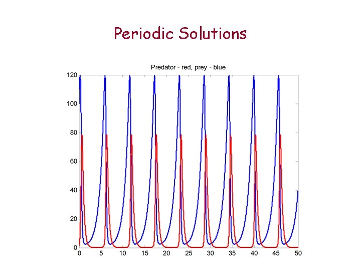
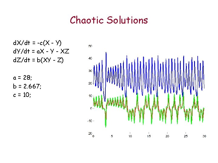
Plan We will learn in this tutorial: translating biological knowledge to differential equations models In the afternoon Lab we use matlab to simulate models generate graphs, make predictions, . . . In particular we will model Reactions, Trafficking, Simple infections Participants will also have an opportunity to ‘play’ with more complex models Lotka-Volterra – periodic solutions Lorenz model – chaos

Modeling Biology Driven Models Biology is understood and is translated into equations, reactions, graphs, Data Driven Modeling: Use experimental data only to construct models Main ingredients : Objects: molecules (cytokines/chemokines/. . . ), cells (Macrophages, Neutrophils, . . . ), organs( lymph node, spleen, . . , lung, . . ) Actions: trafficking/migration, interaction (activation/inhibition), proliferation Differential equations are about rate of change of quantities

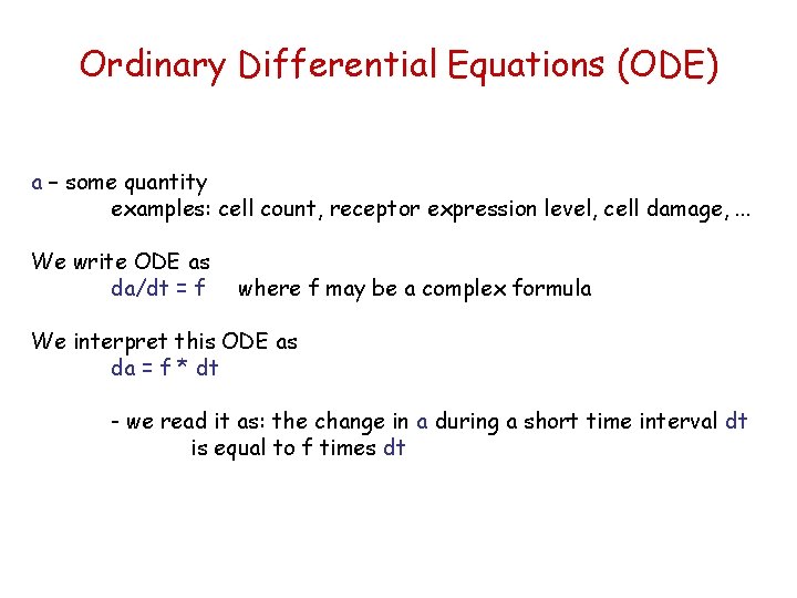
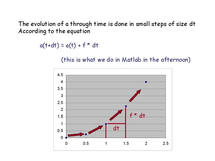
Ordinary Differential Equations (ODE) a – some quantity examples: cell count, receptor expression level, cell damage, . . . We write ODE as da/dt = f where f may be a complex formula We interpret this ODE as da = f * dt - we read it as: the change in a during a short time interval dt is equal to f times dt

The evolution of a through time is done in small steps of size dt According to the equation a(t+dt) = a(t) + f * dt (this is what we do in Matlab in the afternoon) f * dt dt

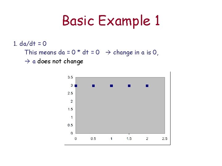
Basic Example 1 1. da/dt = 0 This means da = 0 * dt = 0 change in a is 0, a does not change

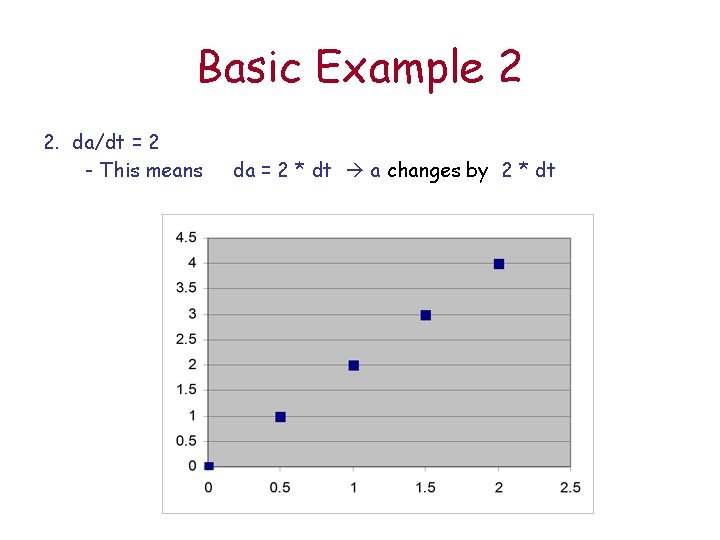
Basic Example 2 2. da/dt = 2 - This means da = 2 * dt a changes by 2 * dt

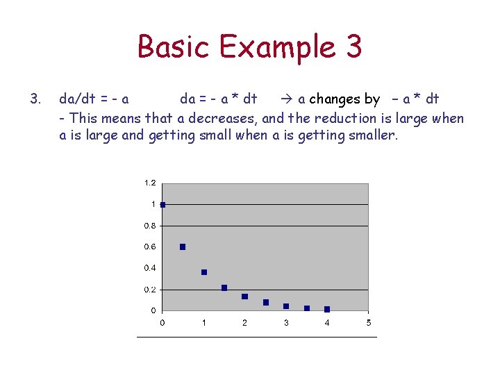
Basic Example 3 3. da/dt = - a da = - a * dt a changes by – a * dt - This means that a decreases, and the reduction is large when a is large and getting small when a is getting smaller.

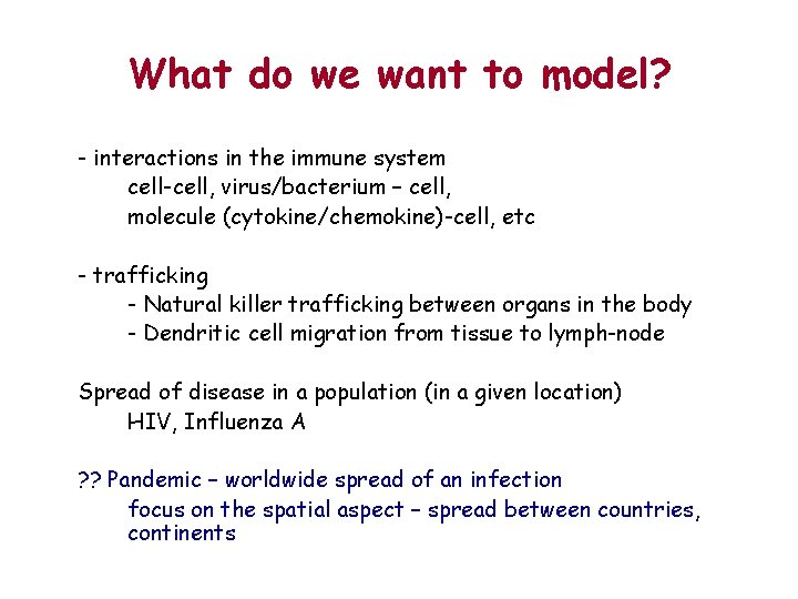
What do we want to model? - interactions in the immune system cell-cell, virus/bacterium – cell, molecule (cytokine/chemokine)-cell, etc - trafficking - Natural killer trafficking between organs in the body - Dendritic cell migration from tissue to lymph-node Spread of disease in a population (in a given location) HIV, Influenza A ? ? Pandemic – worldwide spread of an infection focus on the spatial aspect – spread between countries, continents

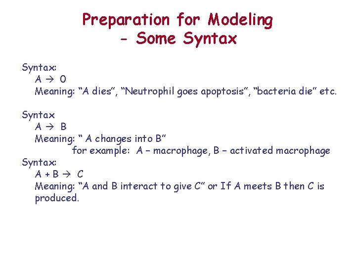
Preparation for Modeling - Some Syntax: A 0 Meaning: “A dies”, “Neutrophil goes apoptosis”, “bacteria die” etc. Syntax A B Meaning: “ A changes into B” for example: A – macrophage, B – activated macrophage Syntax: A+B C Meaning: “A and B interact to give C” or If A meets B then C is produced.

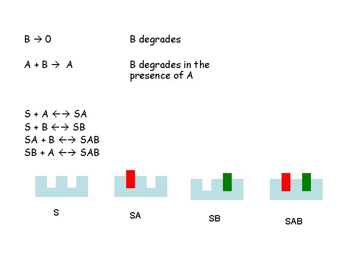
B 0 B degrades A+B A B degrades in the presence of A S + A SA S + B SB SA + B SAB SB + A SAB S SA SB SAB

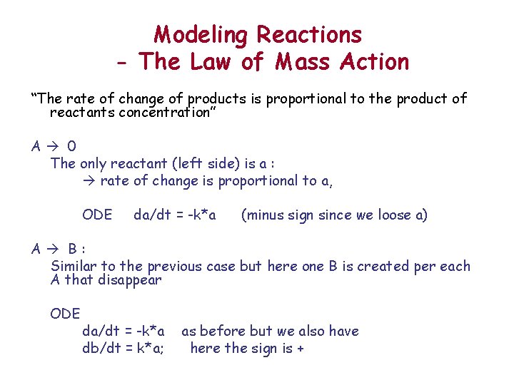
Modeling Reactions - The Law of Mass Action “The rate of change of products is proportional to the product of reactants concentration” A 0 The only reactant (left side) is a : rate of change is proportional to a, ODE da/dt = -k*a (minus sign since we loose a) A B: Similar to the previous case but here one B is created per each A that disappear ODE da/dt = -k*a db/dt = k*a; as before but we also have here the sign is +

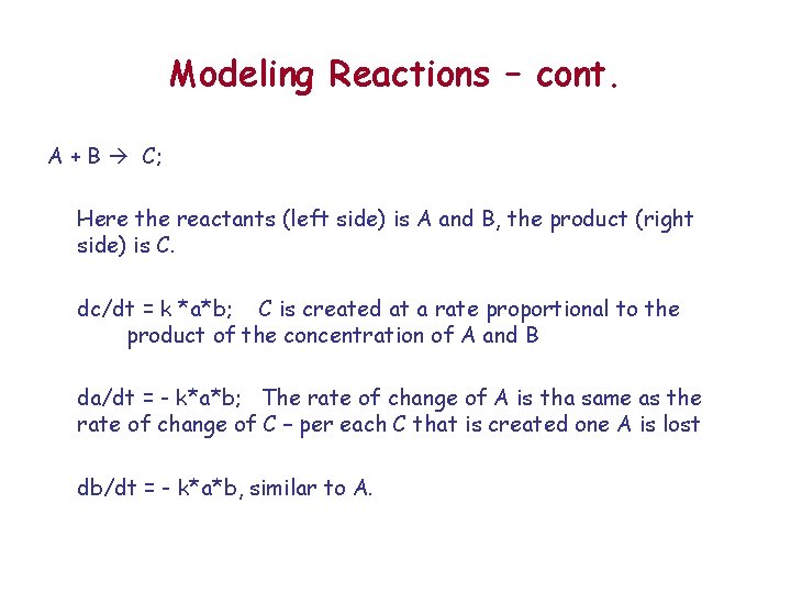
Modeling Reactions – cont. A + B C; Here the reactants (left side) is A and B, the product (right side) is C. dc/dt = k *a*b; C is created at a rate proportional to the product of the concentration of A and B da/dt = - k*a*b; The rate of change of A is tha same as the rate of change of C – per each C that is created one A is lost db/dt = - k*a*b, similar to A.

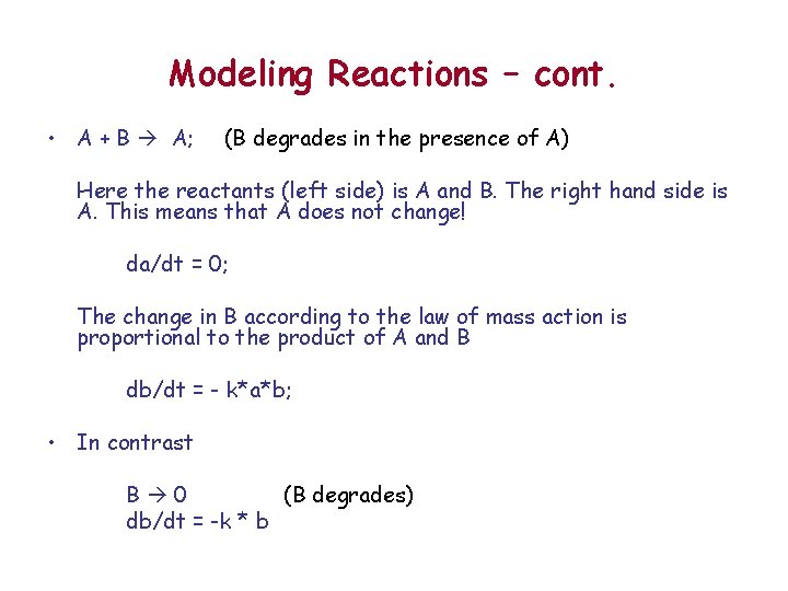
Modeling Reactions – cont. • A + B A; (B degrades in the presence of A) Here the reactants (left side) is A and B. The right hand side is A. This means that A does not change! da/dt = 0; The change in B according to the law of mass action is proportional to the product of A and B db/dt = - k*a*b; • In contrast B 0 (B degrades) db/dt = -k * b

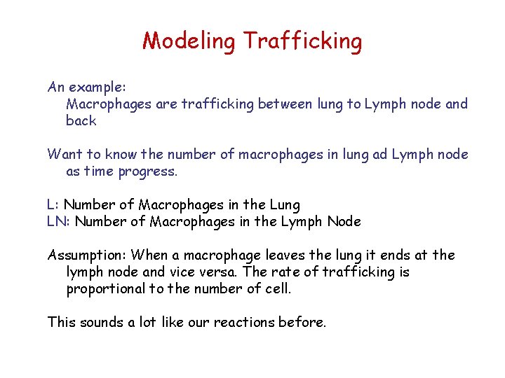
Modeling Trafficking An example: Macrophages are trafficking between lung to Lymph node and back Want to know the number of macrophages in lung ad Lymph node as time progress. L: Number of Macrophages in the Lung LN: Number of Macrophages in the Lymph Node Assumption: When a macrophage leaves the lung it ends at the lymph node and vice versa. The rate of trafficking is proportional to the number of cell. This sounds a lot like our reactions before.

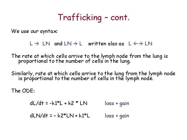
Trafficking – cont. We use our syntax: L LN and LN L written also as L LN The rate at which cells arrive to the lymph node from the lung is proportional to the number of cells in the lung. Similarly, rate at which cells arrive to the lung from the lymph node is proportional to the number of cells in the lymph node. The ODE: d. L/dt = -k 1*L + k 2 * LN loss + gain d. LN/dt = – k 2*LN + k 1*L loss + gain

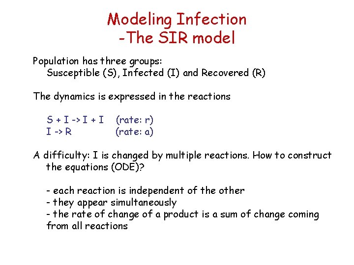
Modeling Infection -The SIR model Population has three groups: Susceptible (S), Infected (I) and Recovered (R) The dynamics is expressed in the reactions S + I -> I + I I -> R (rate: r) (rate: a) A difficulty: I is changed by multiple reactions. How to construct the equations (ODE)? - each reaction is independent of the other - they appear simultaneously - the rate of change of a product is a sum of change coming from all reactions

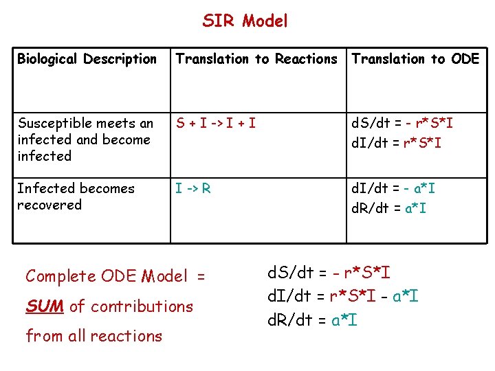
SIR Model Biological Description Translation to Reactions Translation to ODE Susceptible meets an infected and become infected S + I -> I + I d. S/dt = - r*S*I d. I/dt = r*S*I Infected becomes recovered I -> R d. I/dt = - a*I d. R/dt = a*I Complete ODE Model = SUM of contributions from all reactions d. S/dt = - r*S*I d. I/dt = r*S*I - a*I d. R/dt = a*I

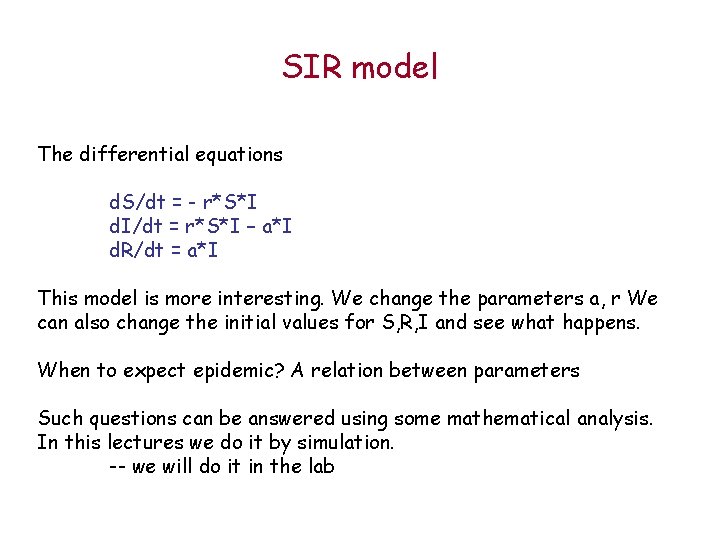
SIR model The differential equations d. S/dt = - r*S*I d. I/dt = r*S*I – a*I d. R/dt = a*I This model is more interesting. We change the parameters a, r We can also change the initial values for S, R, I and see what happens. When to expect epidemic? A relation between parameters Such questions can be answered using some mathematical analysis. In this lectures we do it by simulation. -- we will do it in the lab

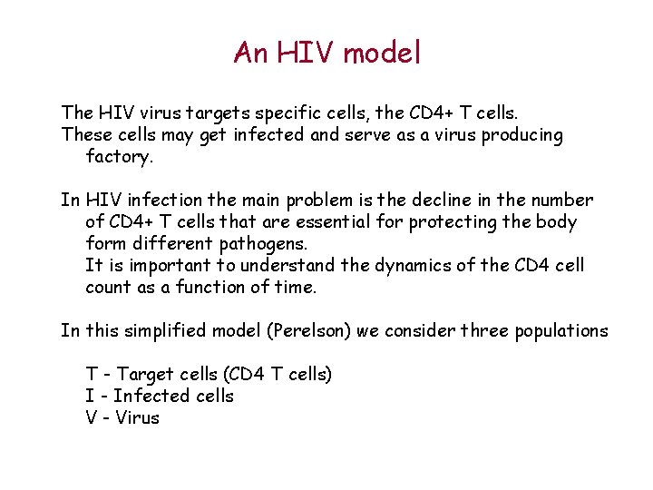
An HIV model The HIV virus targets specific cells, the CD 4+ T cells. These cells may get infected and serve as a virus producing factory. In HIV infection the main problem is the decline in the number of CD 4+ T cells that are essential for protecting the body form different pathogens. It is important to understand the dynamics of the CD 4 cell count as a function of time. In this simplified model (Perelson) we consider three populations T - Target cells (CD 4 T cells) I - Infected cells V - Virus

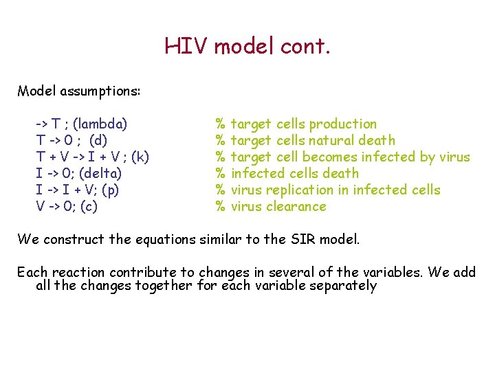
HIV model cont. Model assumptions: -> T ; (lambda) T -> 0 ; (d) T + V -> I + V ; (k) I -> 0; (delta) I -> I + V; (p) V -> 0; (c) % target cells production % target cells natural death % target cell becomes infected by virus % infected cells death % virus replication in infected cells % virus clearance We construct the equations similar to the SIR model. Each reaction contribute to changes in several of the variables. We add all the changes together for each variable separately

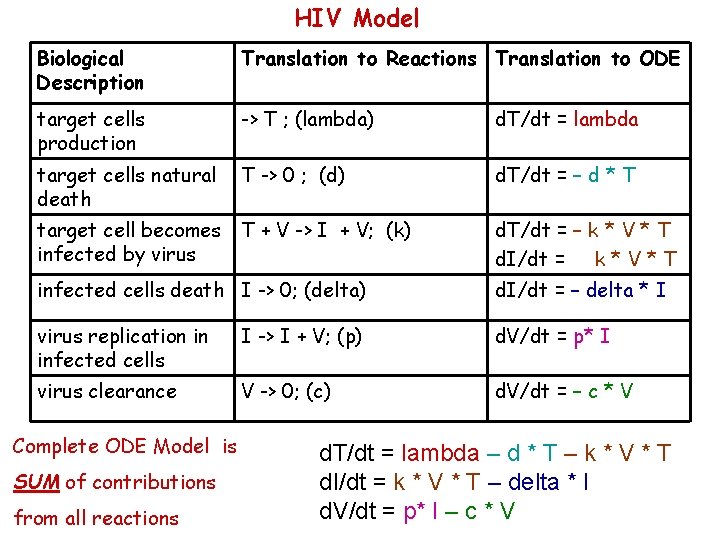
HIV Model Biological Description Translation to Reactions Translation to ODE target cells production -> T ; (lambda) d. T/dt = lambda target cells natural death T -> 0 ; (d) d. T/dt = – d * T target cell becomes infected by virus T + V -> I + V; (k) d. T/dt = – k * V * T d. I/dt = k * V * T infected cells death I -> 0; (delta) d. I/dt = – delta * I virus replication in infected cells I -> I + V; (p) d. V/dt = p* I virus clearance V -> 0; (c) d. V/dt = – c * V Complete ODE Model is SUM of contributions from all reactions d. T/dt = lambda – d * T – k * V * T d. I/dt = k * V * T – delta * I d. V/dt = p* I – c * V

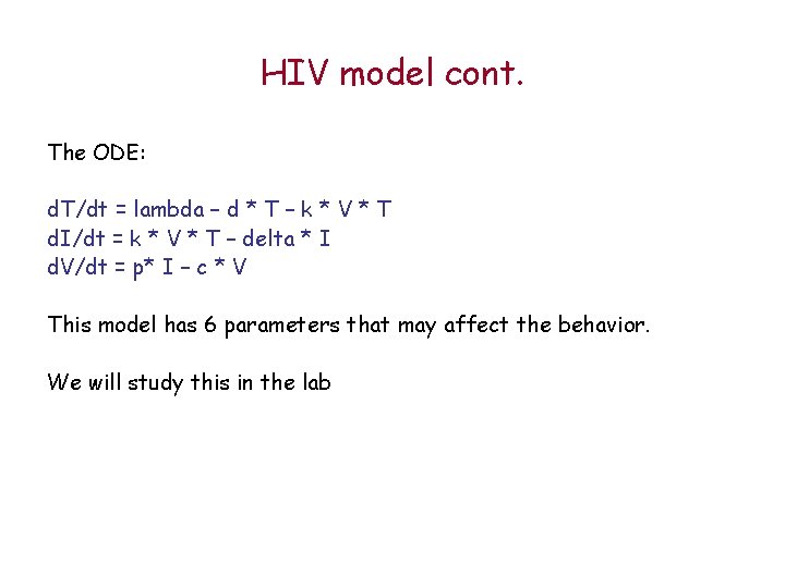
HIV model cont. The ODE: d. T/dt = lambda – d * T – k * V * T d. I/dt = k * V * T – delta * I d. V/dt = p* I – c * V This model has 6 parameters that may affect the behavior. We will study this in the lab

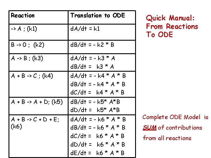
Reaction Translation to ODE -> A ; (k 1) d. A/dt = k 1 B -> 0 ; (k 2) d. B/dt = - k 2 * B A -> B ; (k 3) d. A/dt = - k 3 * A d. B/dt = k 3 * A A + B -> C ; (k 4) d. A/dt = - k 4 * A * B d. B/dt = - k 4 * A * B d. C/dt = k 4 * A * B A + B -> A + D; (k 5) d. B/dt = - k 5* A*B d. D/dt = k 5* A*B A + B -> C + D + E; (k 6) d. A/dt = - k 6 * A * B d. B/dt = - k 6 * A * B d. C/dt = k 6 * A * B d. D/dt = k 6 * A * B d. E/dt = k 6 * A * B Quick Manual: From Reactions To ODE Complete ODE Model is SUM of contributions from all reactions

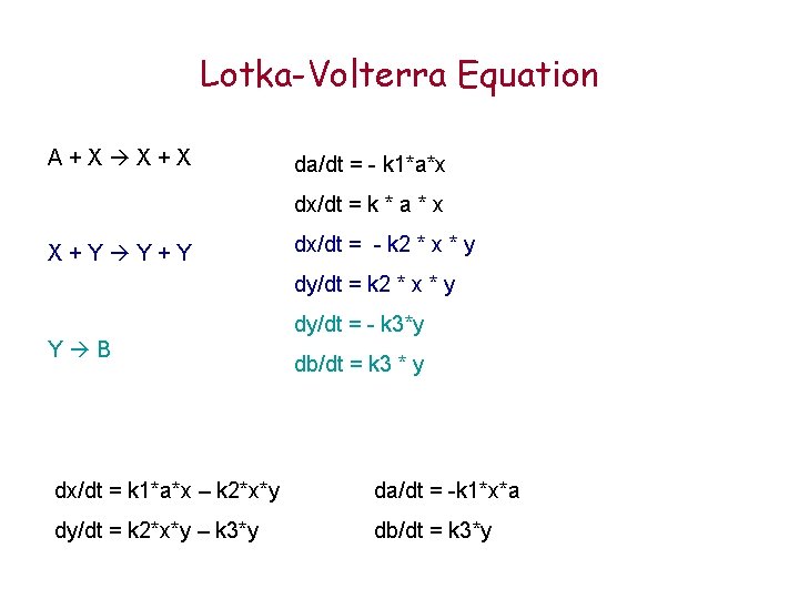
Lotka-Volterra Equation A+X X+X da/dt = - k 1*a*x dx/dt = k * a * x X+Y Y+Y dx/dt = - k 2 * x * y dy/dt = - k 3*y Y B db/dt = k 3 * y dx/dt = k 1*a*x – k 2*x*y da/dt = -k 1*x*a dy/dt = k 2*x*y – k 3*y db/dt = k 3*y

Periodic Solutions

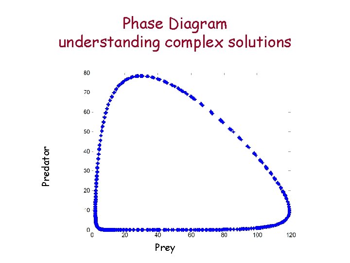
Predator Phase Diagram understanding complex solutions Prey

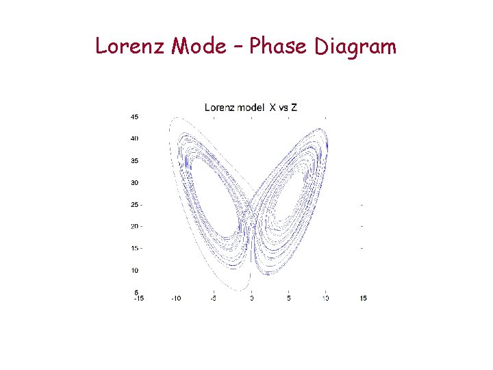
Chaotic Solutions d. X/dt = -c(X - Y) d. Y/dt = a. X - Y - XZ d. Z/dt = b(XY - Z) a = 28; b = 2. 667; c = 10;

Lorenz Mode – Phase Diagram

Now You are Ready to Do Your Own ODE Models • The Question • The Variables • The Interaction/Trafficking/… • Translate to ODE • Simulate • How does …. ? ?

Enjoy!!