Interplay between Optimization and Generalization in DNNs S

Interplay between Optimization and Generalization in DNNs S. Sathiya Keerthi Microsoft (Office-FAST Data Science Team) keerthi@microsoft. com Criteo Workshop on ML in the Real World November 8, 2017, Paris, France DNN = Deep Neural Network References are hyperlinked at appropriate places. Notes in individual slides contain additional comments.
")
DNN Optimization (Training)

Optimization Methods • Let be the Error function to minimize • Weight update: • (Batch) Gradient descent (GD): • We can include gradient-based optimization methods in this class of methods • (Mini-batch) SGD*: • • - B is a mini-batch There exist many variants such as momentum, Adam etc. GD can be viewed as SGD with a large batch Rest of the talk: SGD will simply refer to the plain mini-batch SGD Smaller batch sizes mean more noisy (jumpy) updates *SGD = Stochastic GD

SGD on DNNs Effect of batch size Large batch sizes have an adverse effect on generalization DNN practitioners have been aware of this for more than 5 years. But no clear arguments for why this is so. Goyal et al, ar. Xiv: 1706. 02677
![DNNs & Over-Parametrization [Ref]](http://slidetodoc.com/presentation_image_h/11d2fb98e73a0efc7b1db4b2e5c28579/image-5.jpg "DNNs & Over-Parametrization [Ref]")
DNNs & Over-Parametrization [Ref]

DNNs: Over-parametrization yields great generalization even without any explicit regularization The interesting part – Great generalization! Note the zero training error in the over-parametrized part • • • DNN forms patterns, thus generalizing well It also memorizes noisy examples, but in a harmless way All these need more understanding Zhang et al, Theory of deep learning III, September 2017

More examples of great generalization without any regularization n = number of examples p = number of parameters d = number of inputs k = number of layers Note that networks with larger p/n have better generalization Ben Recht Talk slides, ICLR 2017
![History of powerful DNN solvers on Image. Net (15 million examples) [Ref]](http://slidetodoc.com/presentation_image_h/11d2fb98e73a0efc7b1db4b2e5c28579/image-8.jpg "History of powerful DNN solvers on Image. Net (15 million examples) [Ref]")
History of powerful DNN solvers on Image. Net (15 million examples) [Ref]

In the rest of the talk let’s focus on Over-parametrized systems
![Kernel Methods [Ref]](http://slidetodoc.com/presentation_image_h/11d2fb98e73a0efc7b1db4b2e5c28579/image-10.jpg "Kernel Methods [Ref]")
Kernel Methods [Ref]
 error, • Clean approach")
Standard approach based on regularization • Bound on Generalization (gap) error, • Clean approach to get good generalization by controlling the capacity

In kernel methods, Regularization is sufficient for getting good generalization performance. But is it necessary? Consider an experiment. .

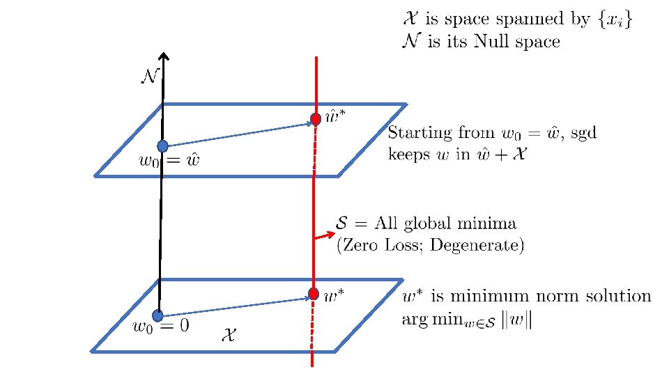
Over-parametrization: SGD + No regularization • Let us consider squared loss: • SGD update: • If we start from then the weight vector at any stage can be written as • SGD can be shown to converge to a minimizer, under suitable control of • Assume X is full rank • Over-parametrization means: • This means: • If we work in kernel feature space and use the kernel trick: • Same as a kernel method moving to zero regularization:

Kernel method with zero regularization gives great performance! Example: On MNIST, with RBF kernel, it gets a test error of 1. 2% which is smaller than that of SVM (1. 4%)

Reason: SGD goes to Minimum Norm Solution • The solution norm solution: is nothing but the minimum • Minimum norm solution also has nice robustness properties – • Insensitivity of the output to input changes • Hence it also has good generalization • That’s a WOW property of SGD – but how did it get it? Let’s try to understand this.

There is nothing special about SGD • We will get minimum norm solution whenever we use any gradient based method and start from • With DNNs, we will see that SGD is indeed special. • But, that comes about not because of the property we are discussing here. • A related note: • Linear case: Hessian* of the empirical loss, E, is constant for quadratic loss. • It is mildly varying for other losses. • In DNNs, the Hessian is highly varying as a function of w. This is an important factor for consideration. *Hessian is the matrix of second order partial derivatives of E with respect to the weights

Over-Parametrized DNNs Some Basic Insights

Understanding via Hessian Properties • Let’s take squared loss for easy analysis: • Gradient: • Hessian: • Note: • When the • Over-parametrized case: the rank of is limited by the number of examples, n • Local minima: have large values - we can expect Hessian to be sharp • Global minima: have small values – Hessian is heavily rank deficient • In the perfect zero error case a global minimum of overparametrized DNNs is degenerate – it is a nonlinear manifold of large dimension • Hessian is dominated by and, it varies a lot across that manifold – this is a property that makes DNNs very different from linear systems • There are numerous such global minimums
 case,")
Ease of reaching a global Minimum • In the lightly over-parametrized (or under-parametrized) case, the error function is lot more sharper • Chances of getting caught in a poor local minimum is higher, especially for a low-noise methods such as GD and SGD with large batch sizes • The time taken to go to a minimum is generally large • Over-parametrized systems do not suffer from such issues • Getting to a global minimum is easy* • Training time is also much shorter *With sigmoid/tanh activations there can be some slow down due to the flat ends, but that can be overcome using good heuristics.
 set of global minima in one basin of attraction is a nonlinear")
The (connected) set of global minima in one basin of attraction is a nonlinear manifold of very high dimension in the zero error case Global minima (Degenerate) Different weight vectors have different Hessian properties Liao and Poggio, Theory of deep learning II, June 2017

Empirical Analysis of SGD Keskar et al did many experiments to understand the effect of batch size on SGD

Large batch yields inferior generalization. . Keskar et al: This is due to flatness properties of solutions This experiment was done on a modified Alex. Net (CNN) on CIFAR-10 dataset

Flatness was first advocated in Hochreiter and Schmidhuber, 1997. Keskar et al’s definition of Sharpness of a solution w (Flatness is the inverse of Sharpness)
 correlates well with sharpness, thus explaining the superiority of small batch over")
Generalization (negatively) correlates well with sharpness, thus explaining the superiority of small batch over large batch Continuous red line: ; Broken red line: This experiment was done on a modified Alex. Net (CNN) on CIFAR-10 dataset

Why flatness means better generalization? Good Bad Flatness implies that the test loss will be close to the training loss
![How does SGD find Flat minima? [Ref]](http://slidetodoc.com/presentation_image_h/11d2fb98e73a0efc7b1db4b2e5c28579/image-27.jpg "How does SGD find Flat minima? [Ref]")
How does SGD find Flat minima? [Ref]

Langevin approximation • SGD: where • Now can be approximated well by a Gaussian which has zero mean and a variance that is proportional to • This yields the (discretized) Langevin system, (SGDL) • The probability distribution associated with this system is the Boltzmann distribution • Large B: Deterministic (not good). Small B: Too noisy (also not good)

A Simple Example 1 2 Frequency histograms of GDL. Note the low values for the sharp minimum An error function with one sharp and one flat global minima 3 It would be interesting to do a better example where flatness changes within one set of degenerate global minima.
 set of global minima in one basin of attraction is a nonlinear")
The (connected) set of global minima in one basin of attraction is a nonlinear manifold of very high dimension in the zero error case Global minima (Degenerate) In the end phase, sgd moves within a region of low loss values and settles in regions with good flatness properties Liao and Poggio, Theory of deep learning II, June 2017 Different weight vectors have different flatness properties

SGD End phase – some conjectures • Gradient size remaining small means • We remain within the basin of one global minimum • Loss values remain small throughout the diffusion phase • The fact that we consistently get good generalization irrespective of random initialization means that • All global minima have flat regions. [Showing/Arguing the existence of such flat regions within each degenerate global minimum is an interesting direction for research. ] • Training algorithms just have to make sure that they move the weight exploration to the flat parts. Clearly, SGD does this so well.

Nailing Flatness Cleanly • For DNNs, Flatness plays a role similar to Margin for kernel methods • Capacity is controlled by the amount of flatness of the weight vector found • A precise definition of flatness using which necessary and sufficient conditions can be given for generalization, is an active topic of research. • Such a definition, if it also lends itself to easy computation, can also act as a regularizer for DNN training. Two examples: • Elastic-SGD: Maximize • Path-SGD: With Rel. U activation, scaling of weights in one layer can be compensated for exactly in a subsequent layer. Path-SGD works with “steepest descent” direction under such scaling invariance. • Continuing our discussion of flatness, let us also connect it to some recent Sensitivity and Information theoretic analysis. .
![Input-Output Sensitivity [Ref]](http://slidetodoc.com/presentation_image_h/11d2fb98e73a0efc7b1db4b2e5c28579/image-33.jpg "Input-Output Sensitivity [Ref]")
Input-Output Sensitivity [Ref]

Sensitivity of Input-Output Map • Sensitivity can be measured as the Frobenius norm of the Input-Output Jacobian of a DNN • Sensitivity has great correlation with Generalization in over-parametrized DNNs • This is not surprising. • When used as a regularizer, its equivalence with data augmentation using input noise injection is well known. • It would be interesting to explore relation between Sensitivity and Flatness. • Would Sensitivity used as a regularizer in the end phase allow large batch gradient methods to generalize equally well as mini-batch SGD?

Sensitivity correlates well with Generalization

Re. LU generalizes getter than Hard. Sigmoid Note again, the correlation between Sensitivity and Generalization
 Note again, the correlation between")
SGD generalizes better than a Full Batch method (BFGS) Note again, the correlation between Sensitivity and Generalization
![Information Bottleneck View [Ref] • • • This work does not give any working](http://slidetodoc.com/presentation_image_h/11d2fb98e73a0efc7b1db4b2e5c28579/image-38.jpg "Information Bottleneck View [Ref] • • • This work does not give any working")
Information Bottleneck View [Ref] • • • This work does not give any working recipes for the practitioner. But it tries to give insights into the working of DNNs and SGD. Paper rejected by both ICML and NIPS this year. But it obtained a lot of press coverage. A recent paper has disputed some key results from this work.

An interesting observation. . • Consider the gradient of the loss with respect to the weights • Phase 1 (Drift) – Mean gradient size is much larger than the standard deviation • Phase 2 (Diffusion) – Mean gradient is smaller and noise takes over (the magic of Langevin comes here) – Langevin/Boltzmann effect kicks in here

The controversy. . • Shwartz-Ziv and Tishby claimed that SGD training compresses (reduces I(X; T)) in the diffusion phase • This has been countered by a recent submission to ICLR that points out that the compression is an artifact of binning associated with tanh neuron outputs.

DNNs being tolerant of Over-parametrization – Does it mean is a Reality? No, not necessarily!

Training error Testing error Training set is large means the two error curves are close to each other. Combined with flatness this yields good generalization Training set is small means the two error curves are away from each other. Even with good flatness this may mean bad generalization

Final Comments
 mini-batch generalize well • Analysis of similar")
Summary • Over-parametrized DNNs trained using (not-so-large) mini-batch generalize well • Analysis of similar observation on kernel methods does not explain what happens in DNNs • Where an optimization algorithm lands in a complex region of low error values decides generalization • Good generalizing regions are associated with flatness • The diffusion phase of SGD is crucial for going to flatness regions

Final comments • Noise in training is necessary to generalize well • SGD does well, fine! But • Variants such as plain mini-batch SGD, Adam etc. behave differently • Also, SGD is not designed with generalization in mind • So, it is an uneasy feeling to remain satisfied just knowing SGD does well • Better understanding of the following are needed • • Structure of degenerate global minima, Properties of the nearby low error region, What precisely causes good generalization to happen, and Quantify Flatness so as to correlate it well with Generalization • Come up with regularizers such that minimization of the regularized loss pushes weights to good generalizing solutions • If there are many such good solutions, can Bayesian averaging be explored using a Flatness-based posterior?

Questions?
- Slides: 46