Intermediate Applied Statistics STAT 460 Lecture 19 11102004

Intermediate Applied Statistics STAT 460 Lecture 19, 11/10/2004 Instructor: Aleksandra (Seša) Slavković sesa@stat. psu. edu TA: Wang Yu wangyu@stat. psu. edu

Revised schedule Nov 8 lab on 2 -way ANOVA Nov 10 lecture on two-way ANOVA and blocking Nov 12 lecture repeated measure and review Post HW 9 Nov 15 lab on repeated measures Nov 17 lecture on categorical data/logistic regression HW 9 due Post HW 10 Nov 19 lecture on categorical data/logistic regression Nov 22 lab on logistic regression & project II introduction No class Thanksgiving Nov 29 lab Dec 1 lecture HW 10 due Post HW 11 Dec 3 lecture and Quiz Dec 6 lab Dec 8 lecture HW 11 due Dec 10 lecture & project II due Dec 13 Project II due

Last lecture o Repeated Measures

This lecture o o o Project I Grades Categorical Response (ch. 18, 19, 20)

Common Issues in Project I o Technical n n n o Use of wrong method for the data Not checking the assumptions Not identifying population/sample, observational study/experiment EDA (center, spread, shape, outliers) Considering plus and minuses of the approach Writing/Organization n n No consideration of audience Executive summary (e. g. too much info/too technical) EDA = Exploratory Data Analysis Unlabeled figures No discussion of future work

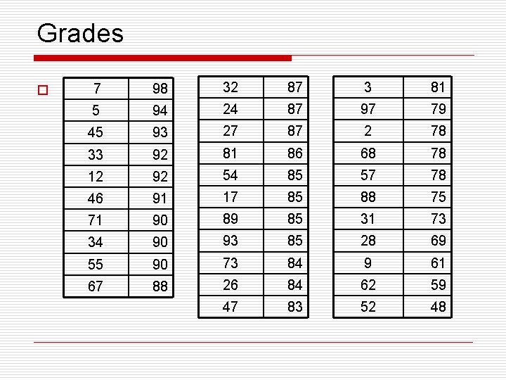
Grades o 7 98 32 87 3 81 5 94 24 87 97 79 45 93 27 87 2 78 33 92 81 86 68 78 12 92 54 85 57 78 46 91 17 85 88 75 71 90 89 85 31 73 34 90 93 85 28 69 55 90 73 84 9 61 67 88 26 84 62 59 47 83 52 48

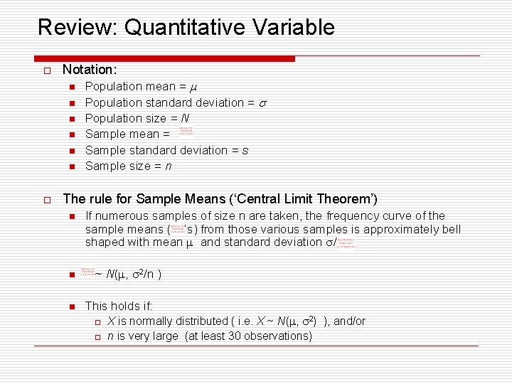
Review: Quantitative Variable o Notation: n n n o Population mean = Population standard deviation = Population size = N Sample mean = Sample standard deviation = s Sample size = n The rule for Sample Means (‘Central Limit Theorem’) n n n If numerous samples of size n are taken, the frequency curve of the sample means ( ‘s) from those various samples is approximately bell shaped with mean and standard deviation / ~ N( , 2/n ) This holds if: o o X is normally distributed ( i. e. X ~ N( , 2) ), and/or n is very large (at least 30 observations)

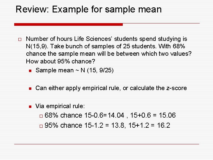
Review: Example for sample mean o Number of hours Life Sciences’ students spend studying is N(15, 9). Take bunch of samples of 25 students. With 68% chance the sample mean will be between which two values? How about 95% chance? n Sample mean ~ N (15, 9/25) n Can either apply empirical rule, or calculate the z-score n Via empirical rule: 68% chance 15 -0. 6=14. 04 , 15+0. 6 = 15. 06 o 95% chance 15 -1. 2 = 13. 8, 15+1. 2 = 16. 2 o

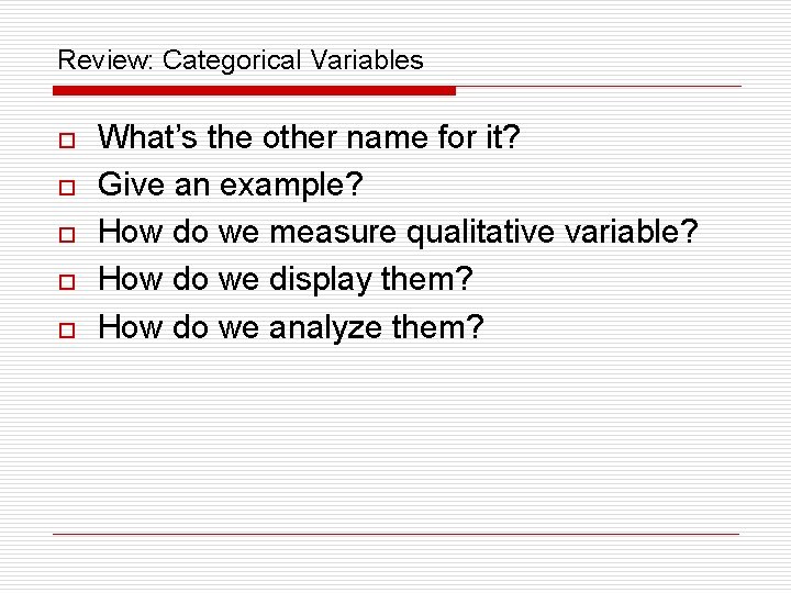
Review: Categorical Variables o o o What’s the other name for it? Give an example? How do we measure qualitative variable? How do we display them? How do we analyze them?

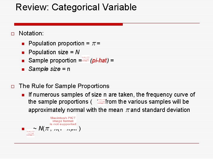
Review: Categorical Variable o Notation: n n o Population proportion = = Population size = N Sample proportion = (pi-hat) = Sample size = n The Rule for Sample Proportions n If numerous samples of size n are taken, the frequency curve of the sample proportions ( ‘s) from the various samples will be approximately normal with the mean and standard deviation n ~ N( , (1 - )/n )

Examples of where the rule of sample proportions apply o o o Polls TV Ratings Consumer Preferences Gingko example Etc.

Example o An advertising agency has stated that 20% of all television viewers watch a particular program. In a random sample of 1000 viewers, x = 184 viewers were watching the program. Do these data present sufficient evidence to contradict the advertiser's claim?

Review: Confidence Interval o o o Empirical rule: 95% chance that the sample proportion is between (0. 174, 0. 226) Mean 2 st. dev We just created a 95% confidence interval This means we are almost sure that values computed from the sample cover the true population value. That is, in 95% of our samples the true proportion (p) will fall within 2 st. dev. of the sample proportion ( p-hat ) Recall, margin of error (MOE) 95% confidence interval for the proportions: n n Sample proportion margin of error p-hat 1/ n

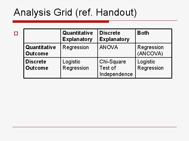
Analysis Grid (ref. Handout) Quantitative Explanatory Discrete Explanatory Both Quantitative Outcome Regression ANOVA Regression (ANCOVA) Discrete Outcome Logistic Regression Chi-Square Logistic Test of Regression Independence o

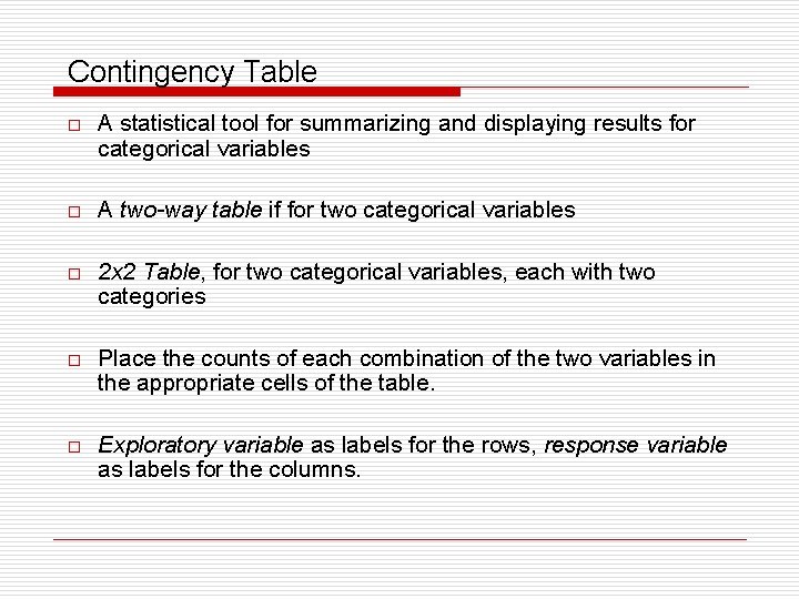
Contingency Table o A statistical tool for summarizing and displaying results for categorical variables o A two-way table if for two categorical variables o 2 x 2 Table, for two categorical variables, each with two categories o Place the counts of each combination of the two variables in the appropriate cells of the table. o Exploratory variable as labels for the rows, response variable as labels for the columns.

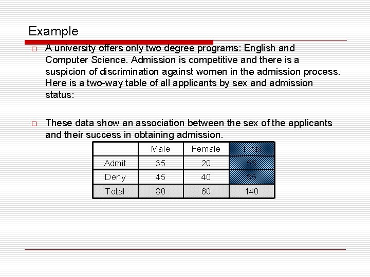
Example o A university offers only two degree programs: English and Computer Science. Admission is competitive and there is a suspicion of discrimination against women in the admission process. Here is a two-way table of all applicants by sex and admission status: o These data show an association between the sex of the applicants and their success in obtaining admission. Male Female Total Admit 35 20 55 Deny 45 40 85 Total 80 60 140

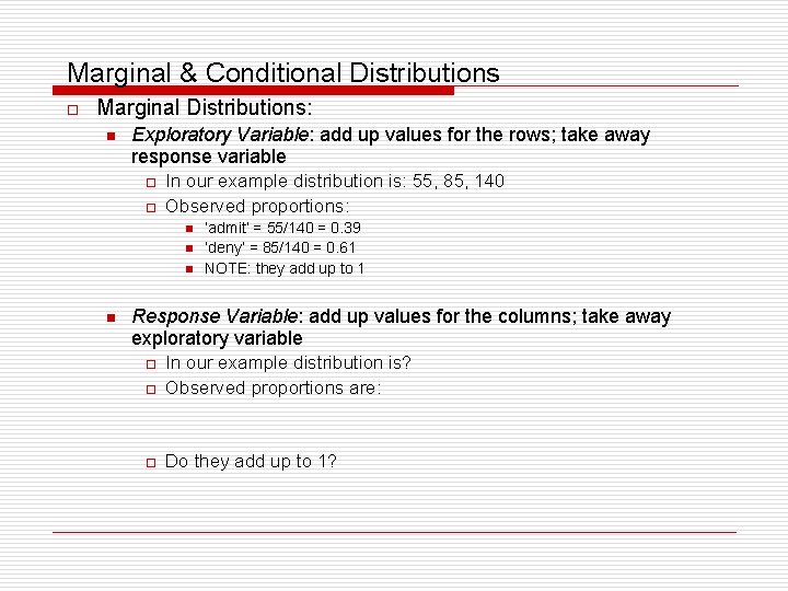
Marginal & Conditional Distributions o Marginal Distributions: n Exploratory Variable: add up values for the rows; take away response variable o o In our example distribution is: 55, 85, 140 Observed proportions: n n ‘admit’ = 55/140 = 0. 39 ‘deny’ = 85/140 = 0. 61 NOTE: they add up to 1 Response Variable: add up values for the columns; take away exploratory variable o In our example distribution is? Observed proportions are: o Do they add up to 1? o

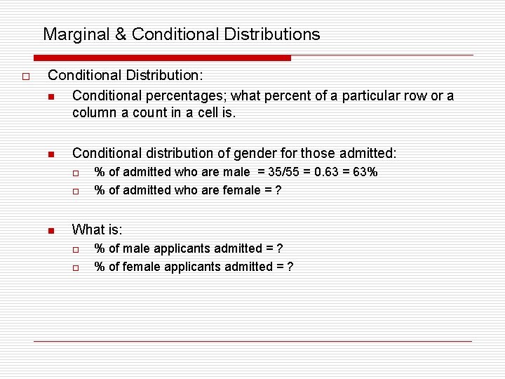
Marginal & Conditional Distributions o Conditional Distribution: n Conditional percentages; what percent of a particular row or a column a count in a cell is. n Conditional distribution of gender for those admitted: o o n % of admitted who are male = 35/55 = 0. 63 = 63% % of admitted who are female = ? What is: o o % of male applicants admitted = ? % of female applicants admitted = ?

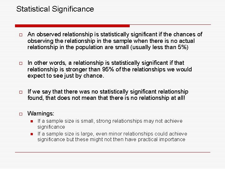
Statistical Significance o An observed relationship is statistically significant if the chances of observing the relationship in the sample when there is no actual relationship in the population are small (usually less than 5%) o In other words, a relationship is statistically significant if that relationship is stronger than 95% of the relationships we would expect to see just by chance. o If we say that there was no statistically significant relationship found, that does not mean that there is no relationship at all! o Warnings: n n If a sample size is small, strong relationships may not achieve significance If a sample size is large, even minor relationships could achieve significance but these might not then have practical importance

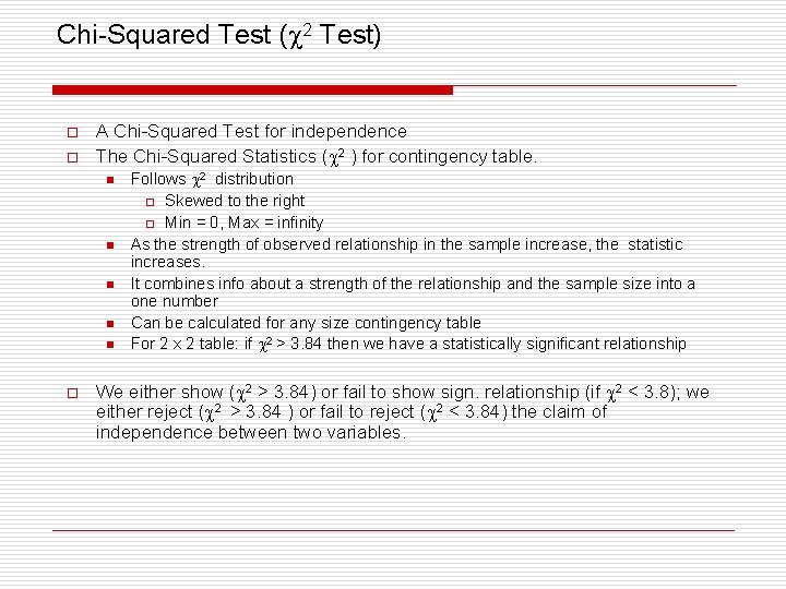
Chi-Squared Test ( 2 Test) o o A Chi-Squared Test for independence The Chi-Squared Statistics ( 2 ) for contingency table. n n n o Follows 2 distribution o Skewed to the right o Min = 0, Max = infinity As the strength of observed relationship in the sample increase, the statistic increases. It combines info about a strength of the relationship and the sample size into a one number Can be calculated for any size contingency table For 2 x 2 table: if 2 > 3. 84 then we have a statistically significant relationship We either show ( 2 > 3. 84) or fail to show sign. relationship (if 2 < 3. 8); we either reject ( 2 > 3. 84 ) or fail to reject ( 2 < 3. 84) the claim of independence between two variables.

2 o o The chi-squared distribution with k-1 degrees of freedom acts as though it was the sum the squares of k-1 independent Normal(0, 1) distributions. (Not that you need to know. ) See table on pages 1100 -1101 in textbook.

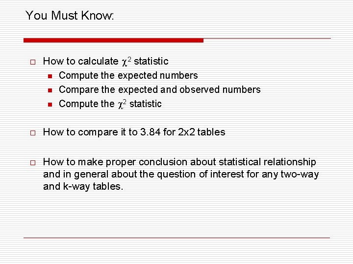
You Must Know: o How to calculate 2 statistic n Compute the expected numbers n Compare the expected and observed numbers n Compute the 2 statistic o How to compare it to 3. 84 for 2 x 2 tables o How to make proper conclusion about statistical relationship and in general about the question of interest for any two-way and k-way tables.

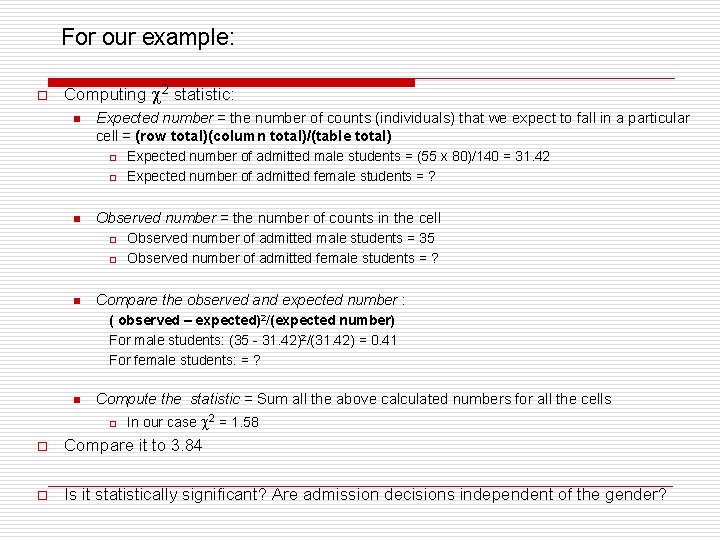
For our example: o Computing 2 statistic: n Expected number = the number of counts (individuals) that we expect to fall in a particular cell = (row total)(column total)/(table total) o o n Observed number = the number of counts in the cell o o n Expected number of admitted male students = (55 x 80)/140 = 31. 42 Expected number of admitted female students = ? Observed number of admitted male students = 35 Observed number of admitted female students = ? Compare the observed and expected number : ( observed – expected)2/(expected number) For male students: (35 - 31. 42)2/(31. 42) = 0. 41 For female students: = ? n Compute the statistic = Sum all the above calculated numbers for all the cells o In our case 2 = 1. 58 o Compare it to 3. 84 o Is it statistically significant? Are admission decisions independent of the gender?

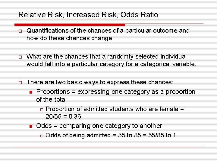
Relative Risk, Increased Risk, Odds Ratio o Quantifications of the chances of a particular outcome and how do these chances change o What are the chances that a randomly selected individual would fall into a particular category for a categorical variable. o There are two basic ways to express these chances: n Proportions = expressing one category as a proportion of the total o Proportion of admitted students who are female = 20/55 = 0. 36 n Odds = comparing one category to another o Odds of being admitted = 55 to 85 = 55/85 to 1

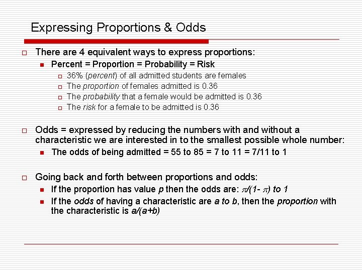
Expressing Proportions & Odds o There are 4 equivalent ways to express proportions: n Percent = Proportion = Probability = Risk o o o Odds = expressed by reducing the numbers with and without a characteristic we are interested in to the smallest possible whole number: n o 36% (percent) of all admitted students are females The proportion of females admitted is 0. 36 The probability that a female would be admitted is 0. 36 The risk for a female to be admitted is 0. 36 The odds of being admitted = 55 to 85 = 7 to 11 = 7/11 to 1 Going back and forth between proportions and odds: n If the proportion has value p then the odds are: /(1 - ) to 1 n If the odds of having a characteristic are a to b, then the proportion with the characteristic is a/(a+b)

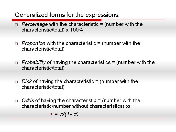
Generalized forms for the expressions: o Percentage with the characteristic = (number with the characteristic/total) x 100% o Proportion with the characteristic = (number with the characteristic/total) o Probability of having the characteristics = (number with the characteristic/total) o Risk of having the characteristic = (number with the characteristic/total) o Odds of having the characteristic = (number with the characteristic/number without characteristics) to 1 § = /(1 - )

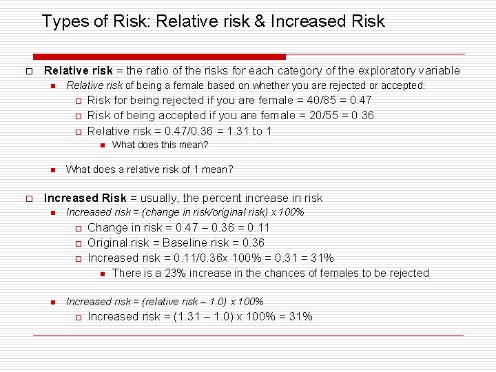
Types of Risk: Relative risk & Increased Risk o Relative risk = the ratio of the risks for each category of the exploratory variable n Relative risk of being a female based on whether you are rejected or accepted: o o o Risk for being rejected if you are female = 40/85 = 0. 47 Risk of being accepted if you are female = 20/55 = 0. 36 Relative risk = 0. 47/0. 36 = 1. 31 to 1 n n o What does this mean? What does a relative risk of 1 mean? Increased Risk = usually, the percent increase in risk n Increased risk = (change in risk/original risk) x 100% o o o Change in risk = 0. 47 – 0. 36 = 0. 11 Original risk = Baseline risk = 0. 36 Increased risk = 0. 11/0. 36 x 100% = 0. 31 = 31% n n There is a 23% increase in the chances of females to be rejected Increased risk = (relative risk – 1. 0) x 100% o Increased risk = (1. 31 – 1. 0) x 100% = 31%

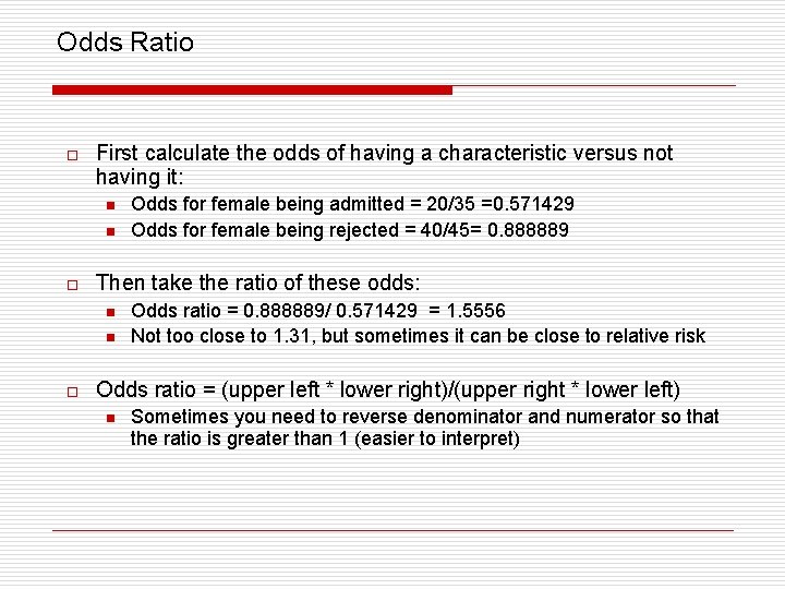
Odds Ratio o First calculate the odds of having a characteristic versus not having it: n n o Then take the ratio of these odds: n n o Odds for female being admitted = 20/35 =0. 571429 Odds for female being rejected = 40/45= 0. 888889 Odds ratio = 0. 888889/ 0. 571429 = 1. 5556 Not too close to 1. 31, but sometimes it can be close to relative risk Odds ratio = (upper left * lower right)/(upper right * lower left) n Sometimes you need to reverse denominator and numerator so that the ratio is greater than 1 (easier to interpret)

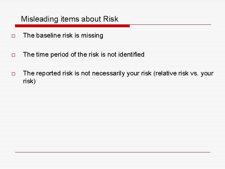
Misleading items about Risk o The baseline risk is missing o The time period of the risk is not identified o The reported risk is not necessarily your risk (relative risk vs. your risk)

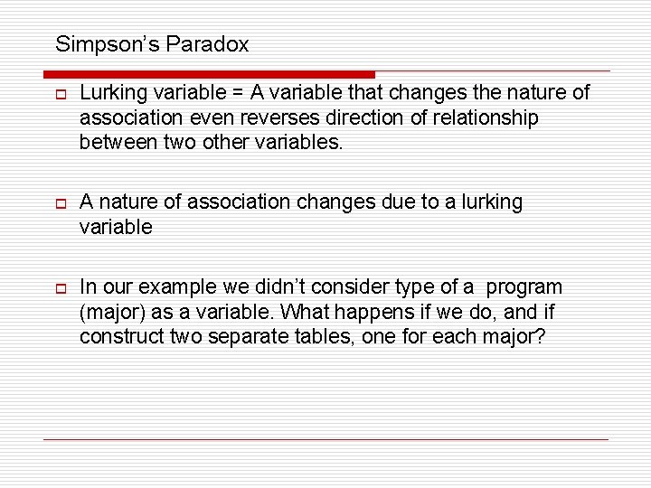
Simpson’s Paradox o Lurking variable = A variable that changes the nature of association even reverses direction of relationship between two other variables. o A nature of association changes due to a lurking variable o In our example we didn’t consider type of a program (major) as a variable. What happens if we do, and if construct two separate tables, one for each major?

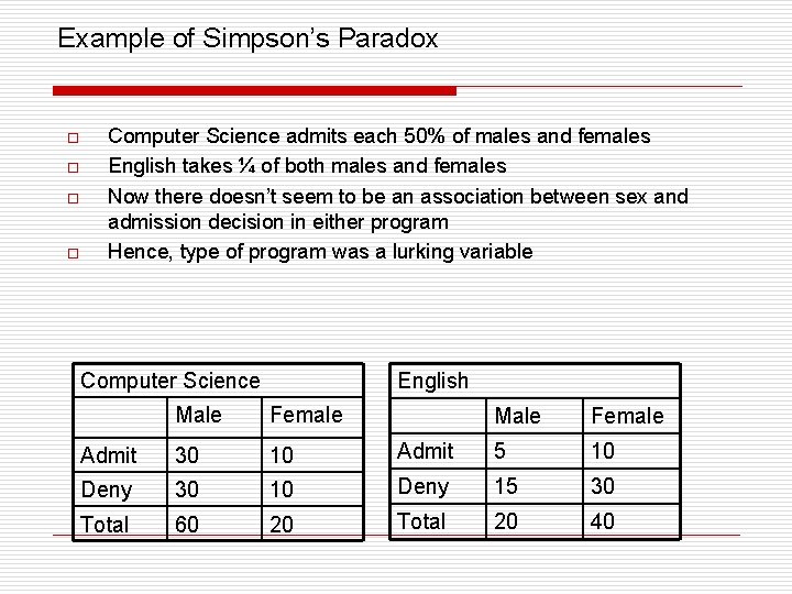
Example of Simpson’s Paradox o o Computer Science admits each 50% of males and females English takes ¼ of both males and females Now there doesn’t seem to be an association between sex and admission decision in either program Hence, type of program was a lurking variable Computer Science English Male Female Admit 30 10 Deny 30 Total 60 Male Female Admit 5 10 10 Deny 15 30 20 Total 20 40

Next o o o Categorical data Logistic regression Lab Monday: Categorical Data, Logistic Regression, Project II