
Introduction to probability Stat 134 FAll 2005 Berkeley
Introduction to probability Stat 134 FAll 2005 Berkeley Lectures prepared by: Elchanan Mossel elena Shvets Follows Jim Pitman’s book: Probability Section 3. 3
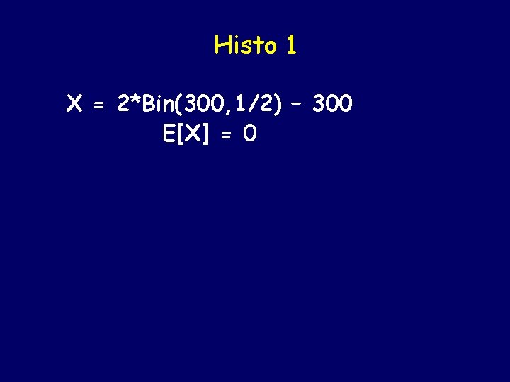
Histo 1 X = 2*Bin(300, 1/2) – 300 E[X] = 0
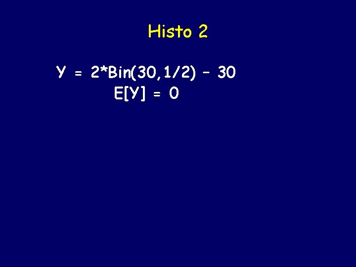
Histo 2 Y = 2*Bin(30, 1/2) – 30 E[Y] = 0
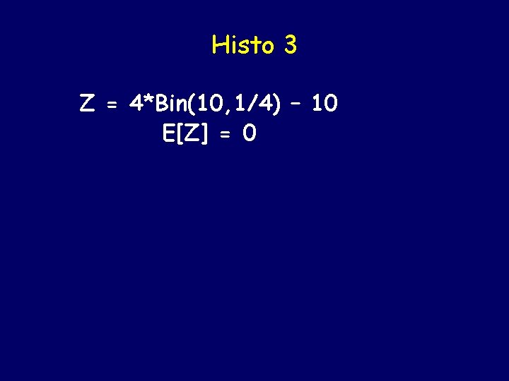
Histo 3 Z = 4*Bin(10, 1/4) – 10 E[Z] = 0
Histo 4 W = 0 E[W] = 0
A natural question: • Is there a good parameter that allow to distinguish between these distributions? • Is there a way to measure the spread?
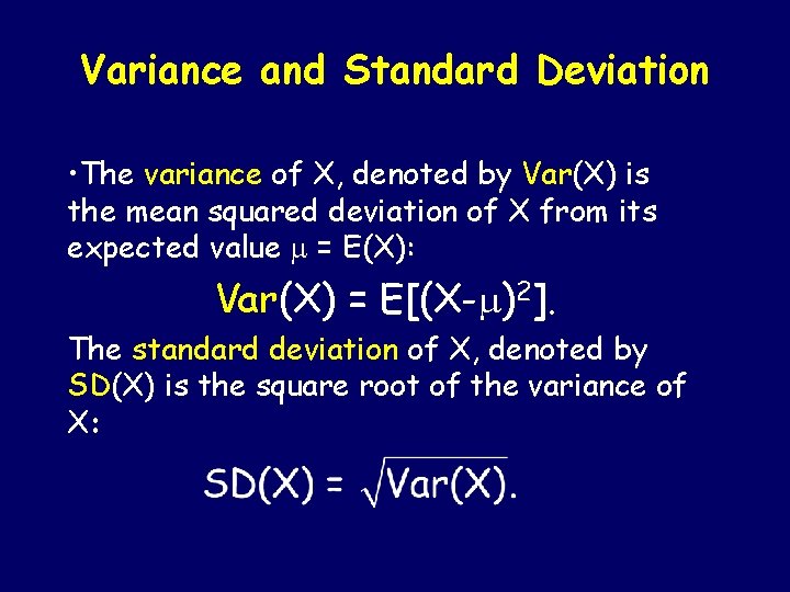
Variance and Standard Deviation • The variance of X, denoted by Var(X) is the mean squared deviation of X from its expected value = E(X): Var(X) = E[(X- )2]. The standard deviation of X, denoted by SD(X) is the square root of the variance of X:
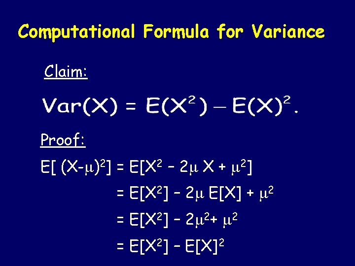
Computational Formula for Variance Claim: Proof: E[ (X- )2] = E[X 2 – 2 X + 2] E[ (X- )2] = E[X 2] – 2 E[X] + 2 E[ (X- )2] = E[X 2] – 2 2+ 2 E[ (X- )2] = E[X 2] – E[X]2
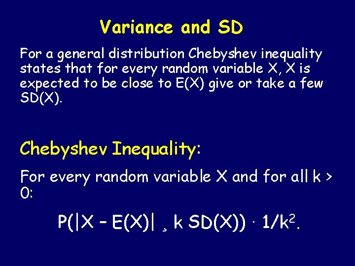
Variance and SD For a general distribution Chebyshev inequality states that for every random variable X, X is expected to be close to E(X) give or take a few SD(X). Chebyshev Inequality: For every random variable X and for all k > 0: P(|X – E(X)| ¸ k SD(X)) · 1/k 2.
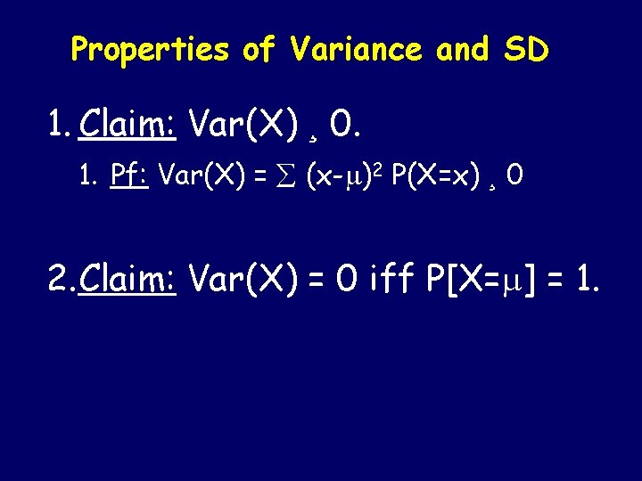
Properties of Variance and SD 1. Claim: Var(X) ¸ 0. 1. Pf: Var(X) = å (x- )2 P(X=x) ¸ 0 2. Claim: Var(X) = 0 iff P[X= ] = 1.
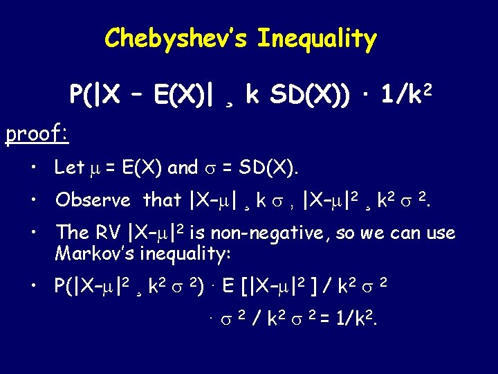
Chebyshev’s Inequality P(|X – E(X)| ¸ k SD(X)) · 1/k 2 proof: • Let = E(X) and = SD(X). • Observe that |X– | ¸ k , |X– |2 ¸ k 2 2. • The RV |X– |2 is non-negative, so we can use Markov’s inequality: • P(|X– |2 ¸ k 2 2) · E [|X– |2 ] / k 2 2 P(|X– |2 ¸ k 2 2) · 2 / k 2 2 = 1/k 2.
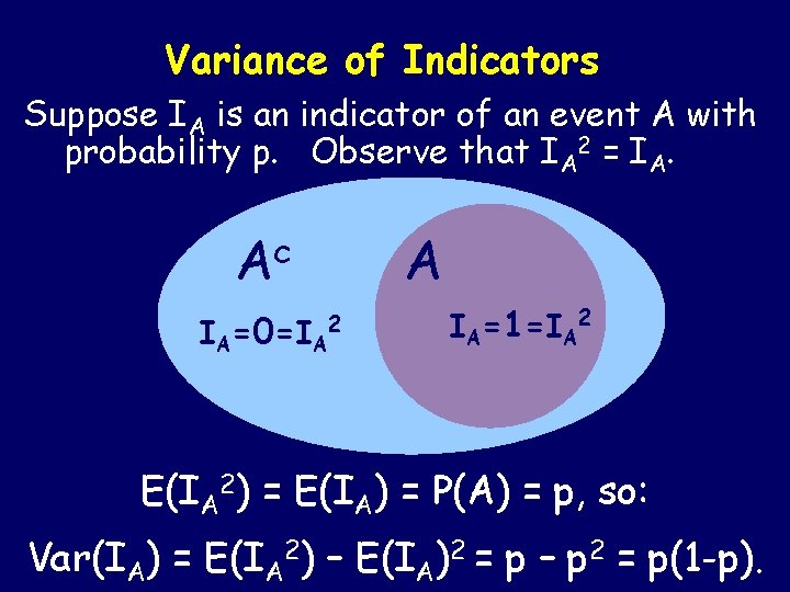
Variance of Indicators Suppose IA is an indicator of an event A with probability p. Observe that IA 2 = IA. Ac IA=0=IA A 2 IA=1=IA 2 E(IA 2) = E(IA) = P(A) = p, so: Var(IA) = E(IA 2) – E(IA)2 = p – p 2 = p(1 -p).
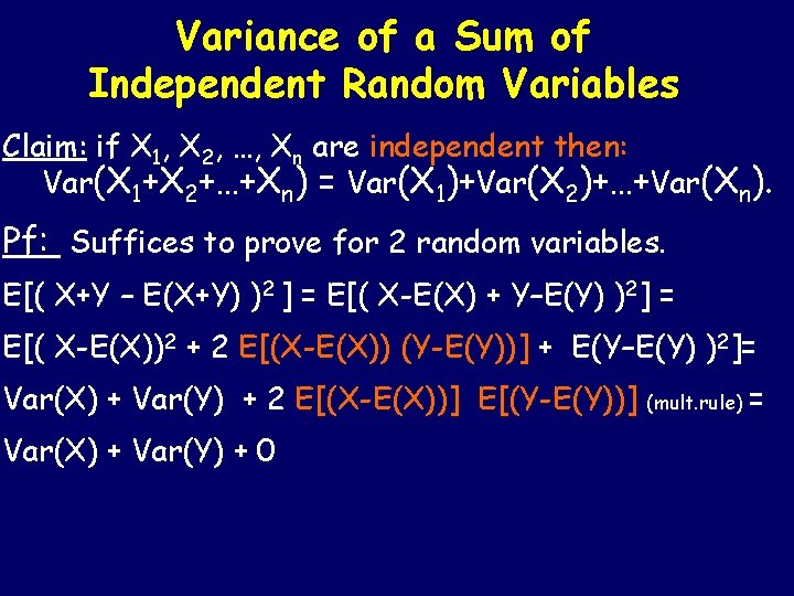
Variance of a Sum of Independent Random Variables Claim: if X 1, X 2, …, Xn are independent then: Var(X 1+X 2+…+Xn) = Var(X 1)+Var(X 2)+…+Var(Xn). Pf: Suffices to prove for 2 random variables. E[( X+Y – E(X+Y) )2 ] = E[( X-E(X) + Y–E(Y) )2] = E[( X-E(X))2 + 2 E[(X-E(X)) (Y-E(Y))] + E(Y–E(Y) )2]= Var(X) + Var(Y) + 2 E[(X-E(X))] E[(Y-E(Y))] Var(X) + Var(Y) + 0 (mult. rule) =
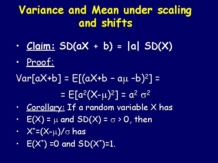
Variance and Mean under scaling and shifts • Claim: SD(a. X + b) = |a| SD(X) • Proof: Var[a. X+b] = E[(a. X+b – a –b)2] = • • = E[a 2(X- )2] = a 2 2 Corollary: If a random variable X has E(X) = and SD(X) = > 0, then X*=(X- )/ has E(X*) =0 and SD(X*)=1.
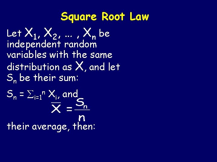
Square Root Law Let X 1, X 2, … , Xn be independent random variables with the same distribution as X, and let Sn be their sum: Sn = åi=1 n Xi, and their average, then:
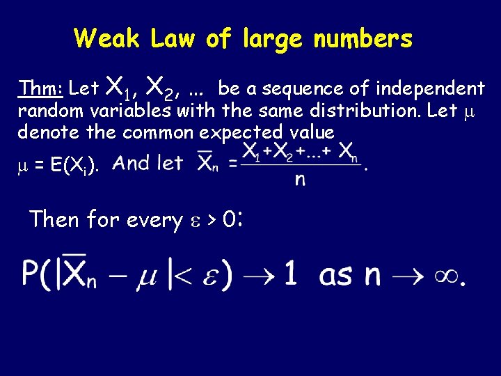
Weak Law of large numbers Thm: Let X 1, X 2, … be a sequence of independent random variables with the same distribution. Let denote the common expected value = E(Xi). Then for every e > 0:
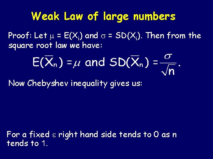
Weak Law of large numbers Proof: Let = E(Xi) and = SD(Xi). Then from the square root law we have: Now Chebyshev inequality gives us: For a fixed e right hand side tends to 0 as n tends to 1.
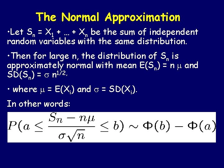
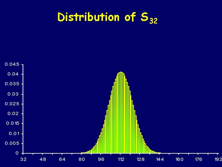
The Normal Approximation • Let Sn = X 1 + … + Xn be the sum of independent random variables with the same distribution. • Then for large n, the distribution of Sn is approximately normal with mean E(Sn) = n and SD(Sn) = n 1/2, • where = E(Xi) and = SD(Xi). In other words:
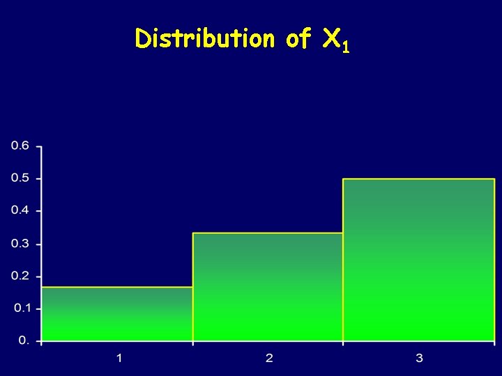
Sums of iid random variables Suppose Xi represents the number obtained on the i’th roll of a die. Then Xi has a uniform distribution on the set {1, 2, 3, 4, 5, 6}.
Distribution of X 1
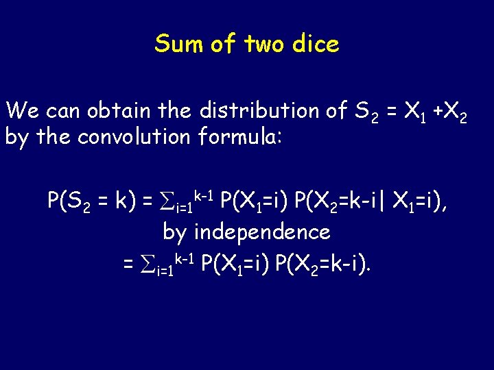
Sum of two dice We can obtain the distribution of S 2 = X 1 +X 2 by the convolution formula: P(S 2 = k) = åi=1 k-1 P(X 1=i) P(X 2=k-i| X 1=i), by independence = åi=1 k-1 P(X 1=i) P(X 2=k-i).
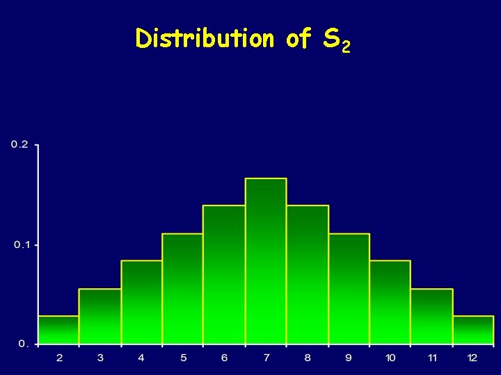
Distribution of S 2
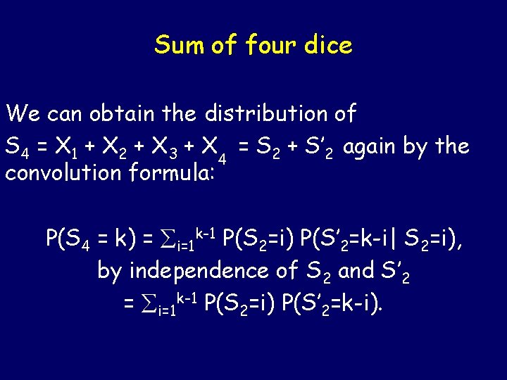
Sum of four dice We can obtain the distribution of S 4 = X 1 + X 2 + X 3 + X 4 = S 2 + S’ 2 again by the convolution formula: P(S 4 = k) = åi=1 k-1 P(S 2=i) P(S’ 2=k-i| S 2=i), by independence of S 2 and S’ 2 = åi=1 k-1 P(S 2=i) P(S’ 2=k-i).
Distribution of S 4
Distribution of S 8
Distribution of S 16
Distribution of S 32
Distribution of X 1
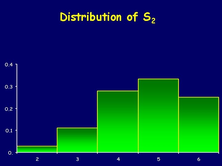
Distribution of S 2
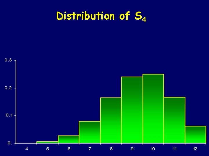
Distribution of S 4
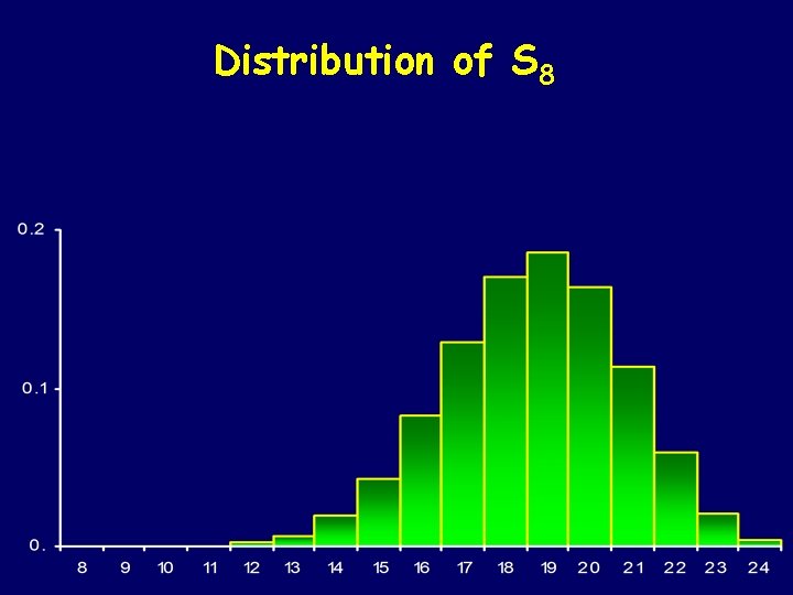
Distribution of S 8
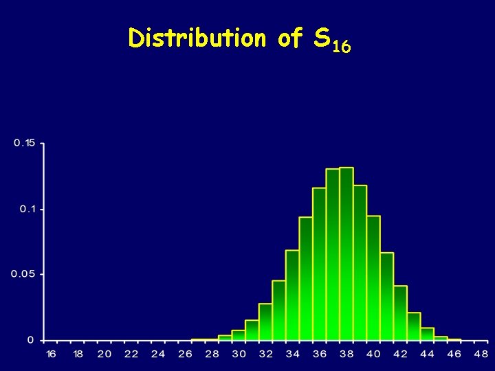
Distribution of S 16
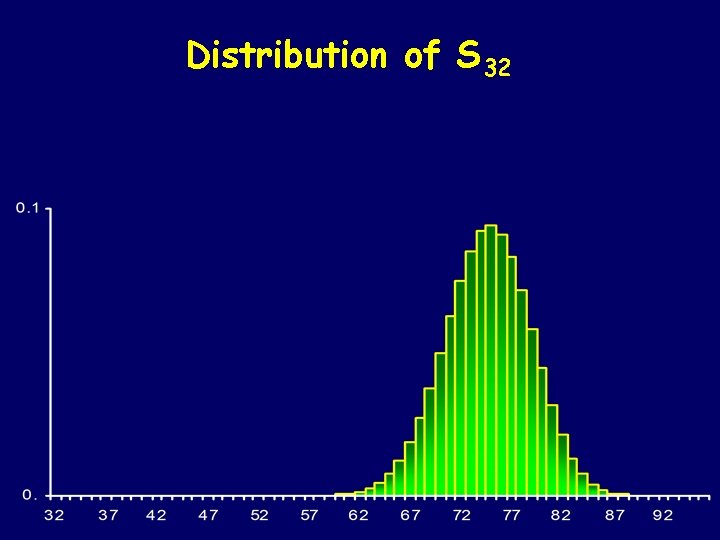
Distribution of S 32
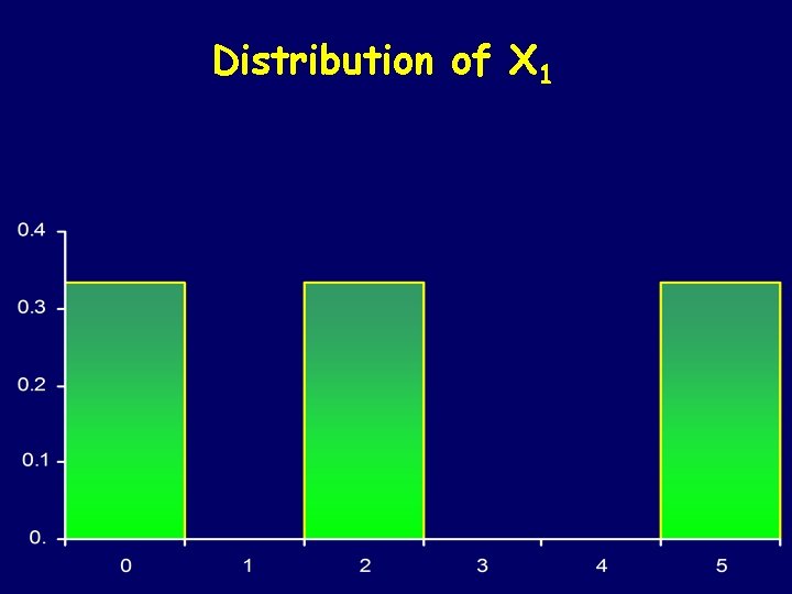
Distribution of X 1
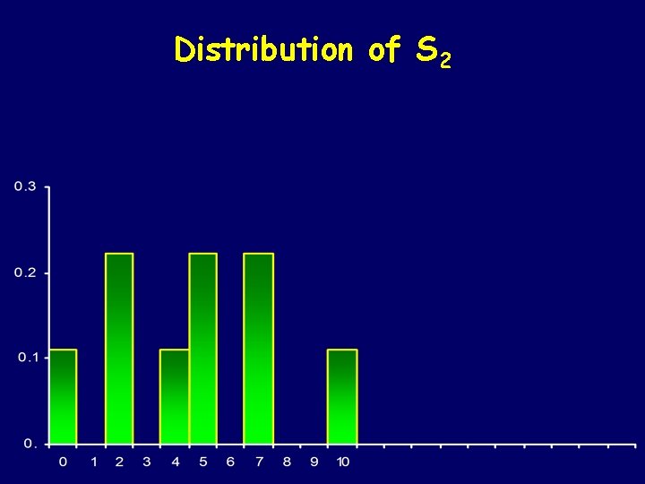
Distribution of S 2
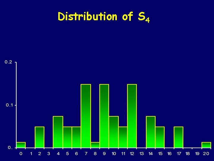
Distribution of S 4
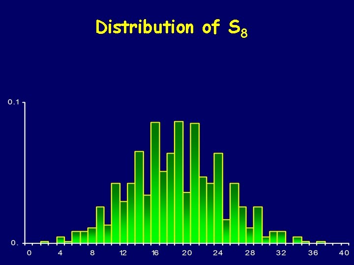
Distribution of S 8
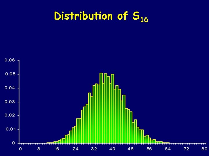
Distribution of S 16
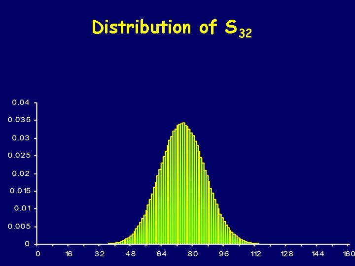
Distribution of S 32
- Slides: 39