III Solution of pdes using integral transforms 3

III Solution of pde’s using integral transforms 3. 1 Introduction • Convolution theorem • Application of Fourier Transforms, Sine and Cosine Transforms • Application of Laplace Transforms

Introduction • Integral transforms are used to: • Simplify solutions by eliminating or reducing order of pde in a particular variable • Offer physical insight into the problem • Convolution (Faltung) theorems • Type of transform depends on BC of problem

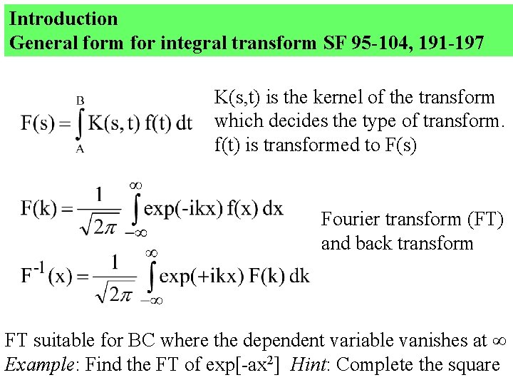
Introduction General form for integral transform SF 95 -104, 191 -197 K(s, t) is the kernel of the transform which decides the type of transform. f(t) is transformed to F(s) Fourier transform (FT) and back transform FT suitable for BC where the dependent variable vanishes at Example: Find the FT of exp[-ax 2] Hint: Complete the square

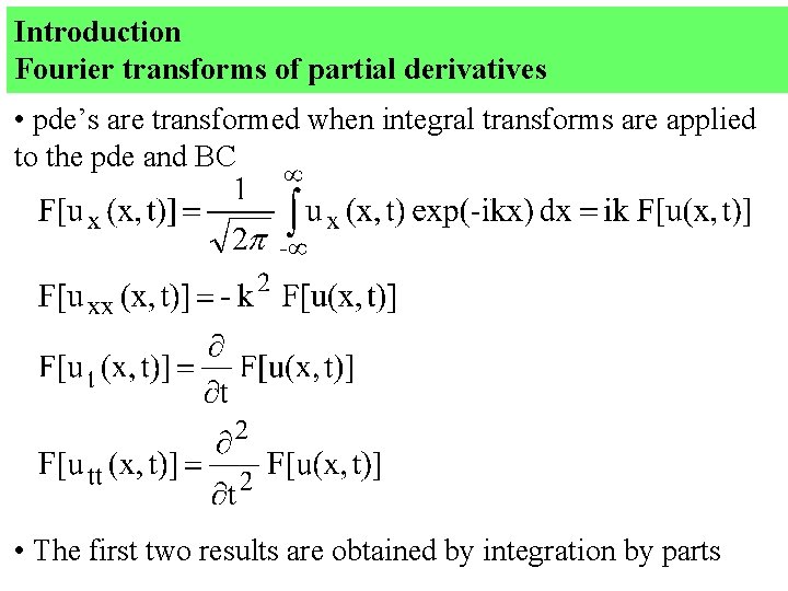
Introduction Fourier transforms of partial derivatives • pde’s are transformed when integral transforms are applied to the pde and BC • The first two results are obtained by integration by parts

Introduction Example: FT the wave equation wrt x utt – c 2 uxx = 0 pde u(x, t) → 0 as x → BC u(x, 0) = exp[-ax 2] IC F[utt] – c 2 F[uxx] = 0 FT pde U''(k, t) + (ck)2 U(k, t) = 0 ode in t U(k, 0) = F[exp(-ax 2)] = FT IC U(k, t) = U(k, 0)exp[–iwt)] u(x, t) = w = ck ode solution pde solution

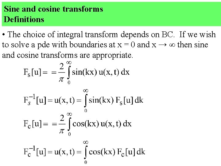
Sine and cosine transforms Definitions • The choice of integral transform depends on BC. If we wish to solve a pde with boundaries at x = 0 and x → then sine and cosine transforms are appropriate.

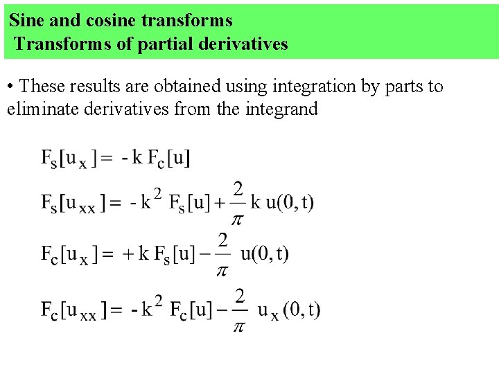
Sine and cosine transforms Transforms of partial derivatives • These results are obtained using integration by parts to eliminate derivatives from the integrand

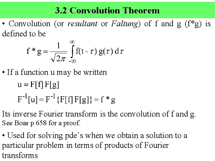
3. 2 Convolution Theorem • Convolution (or resultant or Faltung) of f and g (f*g) is defined to be • If a function u may be written Its inverse Fourier transform is the convolution of f and g. See Boas p 658 for a proof. • Used for solving pde’s when we obtain a solution to a particular problem in terms of products of Fourier transforms

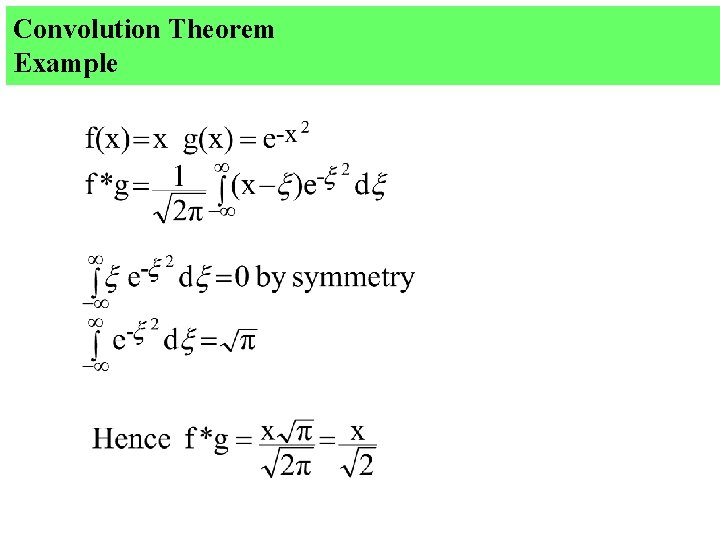
Convolution Theorem Example

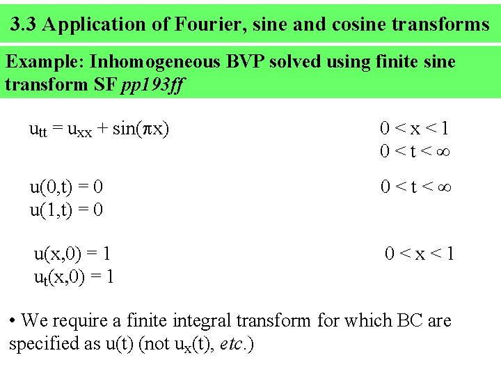
3. 3 Application of Fourier, sine and cosine transforms Example: Inhomogeneous BVP solved using finite sine transform SF pp 193 ff utt = uxx + sin(px) 0 < x < 1 0 < t < u(0, t) = 0 u(1, t) = 0 0 < t < u(x, 0) = 1 ut(x, 0) = 1 0 < x < 1 • We require a finite integral transform for which BC are specified as u(t) (not ux(t), etc. )

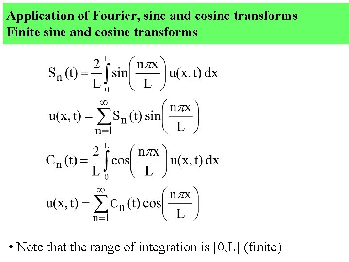
Application of Fourier, sine and cosine transforms Finite sine and cosine transforms • Note that the range of integration is [0, L] (finite)

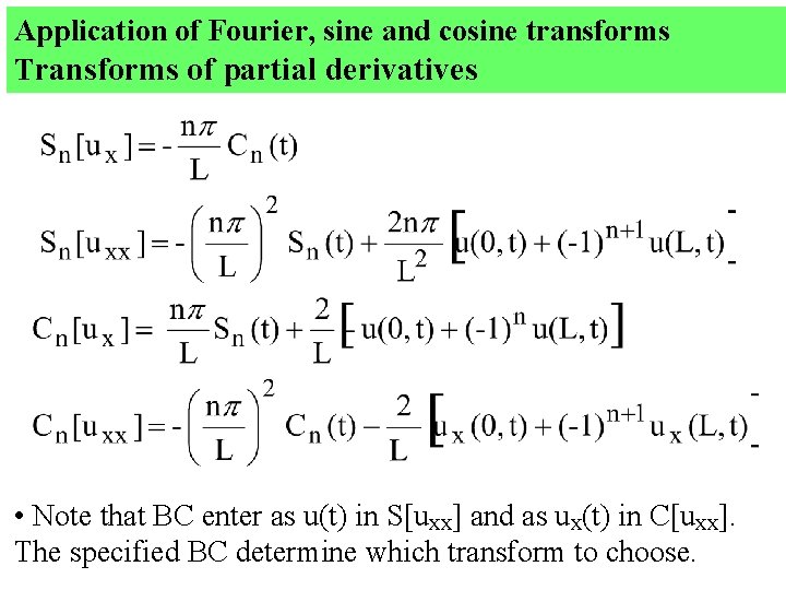
Application of Fourier, sine and cosine transforms Transforms of partial derivatives • Note that BC enter as u(t) in S[uxx] and as ux(t) in C[uxx]. The specified BC determine which transform to choose.

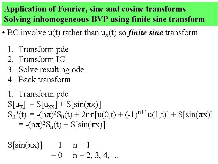
Application of Fourier, sine and cosine transforms Solving inhomogeneous BVP using finite sine transform • BC involve u(t) rather than ux(t) so finite sine transform 1. 2. 3. 4. Transform pde Transform IC Solve resulting ode Back transform 1. Transform pde S[utt] = S[uxx] + S[sin(px)] Sn''(t) = -(np)2 Sn(t) + 2 np[u(0, t) + (-1)n+1 u(1, t)] + S[sin(px)] = -(np)2 Sn(t) + S[sin(px)] = 1 n = 1 = 0 n = 2, 3, 4, …

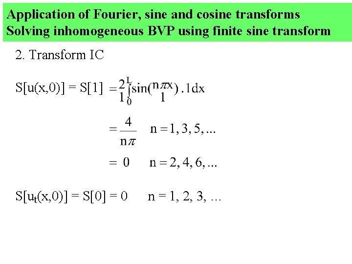
Application of Fourier, sine and cosine transforms Solving inhomogeneous BVP using finite sine transform 2. Transform IC S[u(x, 0)] = S[1] S[ut(x, 0)] = S[0] = 0 n = 1, 2, 3, …

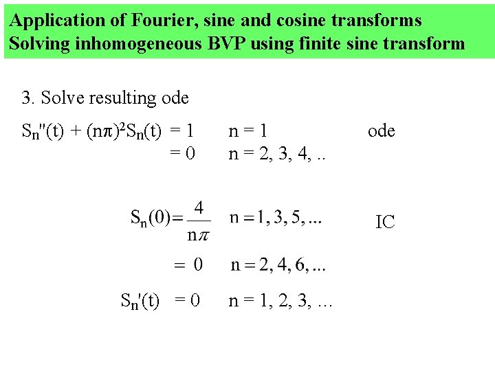
Application of Fourier, sine and cosine transforms Solving inhomogeneous BVP using finite sine transform 3. Solve resulting ode Sn''(t) + (np)2 Sn(t) = 1 = 0 n = 1 n = 2, 3, 4, . . ode IC Sn'(t) = 0 n = 1, 2, 3, …

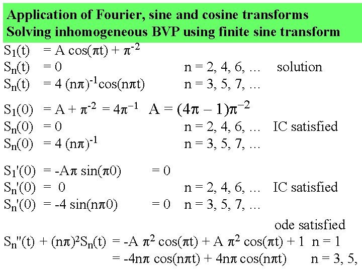
Application of Fourier, sine and cosine transforms Solving inhomogeneous BVP using finite sine transform S 1(t) = A cos(pt) + p-2 Sn(t) = 0 n = 2, 4, 6, … solution Sn(t) = 4 (np)-1 cos(npt) n = 3, 5, 7, … S 1(0) = A + p-2 = 4 p-1 A = (4 p – 1)p-2 Sn(0) = 0 n = 2, 4, 6, … IC satisfied Sn(0) = 4 (np)-1 n = 3, 5, 7, … S 1'(0) = -Ap sin(p 0) Sn'(0) = 0 Sn'(0) = -4 sin(np 0) = 0 n = 2, 4, 6, … IC satisfied = 0 n = 3, 5, 7, … ode satisfied Sn''(t) + (np)2 Sn(t) = -A p 2 cos(pt) + 1 n = 1 = -4 np cos(npt) + 4 np cos(npt) n = 3, 5,

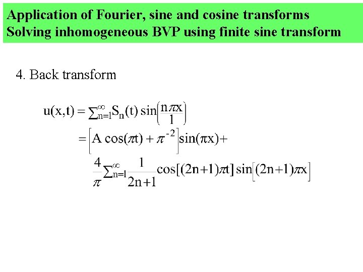
Application of Fourier, sine and cosine transforms Solving inhomogeneous BVP using finite sine transform 4. Back transform

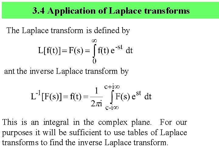
3. 4 Application of Laplace transforms The Laplace transform is defined by ant the inverse Laplace transform by This is an integral in the complex plane. For our purposes it will be sufficient to use tables of Laplace transforms to find the inverse Laplace transform.

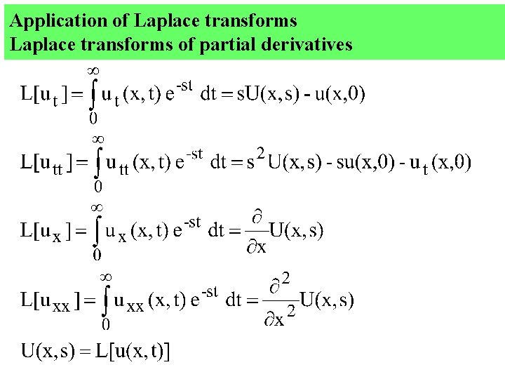
Application of Laplace transforms of partial derivatives

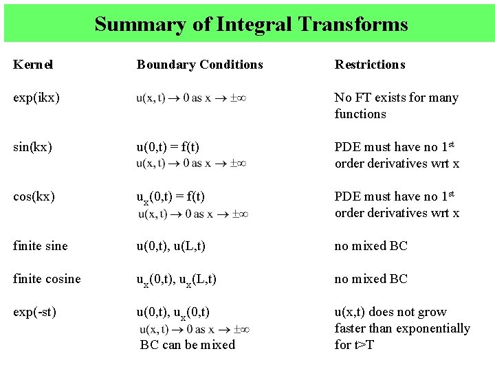
Summary of Integral Transforms Kernel exp(ikx) Boundary Conditions Restrictions No FT exists for many functions sin(kx) u(0, t) = f(t) PDE must have no 1 st order derivatives wrt x cos(kx) ux(0, t) = f(t) PDE must have no 1 st order derivatives wrt x u(0, t), u(L, t) no mixed BC ux(0, t), ux(L, t) no mixed BC u(0, t), ux(0, t) u(x, t) does not grow faster than exponentially for t>T finite sine finite cosine exp(-st) BC can be mixed