FMRI Data Analysis Experiment Design Scanning PreProcessing Individual

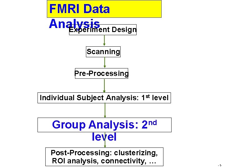
FMRI Data Analysis Experiment Design Scanning Pre-Processing Individual Subject Analysis: 1 st level Group Analysis: 2 nd level Post-Processing: clusterizing, ROI analysis, connectivity, … -1 -

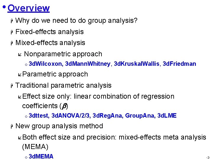
• Overview H Why do we need to do group analysis? H Fixed-effects analysis H Mixed-effects analysis å Nonparametric approach o 3 d. Wilcoxon, åParametric H 3 d. Mann. Whitney, 3 d. Kruskal. Wallis, 3 d. Friedman approach Traditional parametric analysis åEffect size only: linear combination of regression coefficients ( ) o 3 dttest, H 3 d. ANOVA/2/3, 3 d. Reg. Ana, Group. Ana, 3 d. LME New group analysis method åBoth effect size and precision: mixed-effects meta analysis (MEMA) o 3 d. MEMA -2 -

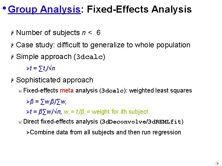
• Group Analysis: Fixed-Effects Analysis H Number of subjects n < 6 H Case study: difficult to generalize to whole population H Simple approach (3 dcalc) Øt H = ∑tii/√n Sophisticated approach å Fixed-effects Øβ Øt meta analysis (3 dcalc): weighted least squares = ∑wiβi/∑wi = β∑wi/√n, wi = ti/βi = weight for ith subject å Direct fixed-effects analysis (3 d. Deconvolve/3 d. REMLfit) ØCombine data from all subjects and then run regression -3 -

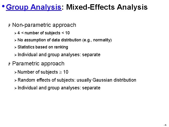
• Group Analysis: Mixed-Effects Analysis H Non-parametric approach Ø 4 < number of subjects < 10 Ø No assumption of data distribution (e. g. , normality) Ø Statistics based on ranking Ø Individual H and group analyses: separate Parametric approach Ø Number Ø Random of subjects 10 effects of subjects: usually Gaussian distribution Ø Individual and group analyses: separate -4 -

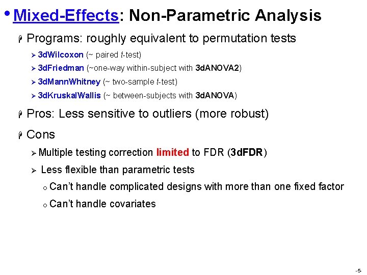
• Mixed-Effects: Non-Parametric Analysis H Programs: roughly equivalent to permutation tests Ø 3 d. Wilcoxon (~ paired t-test) Ø 3 d. Friedman (~one-way within-subject with 3 d. ANOVA 2) Ø 3 d. Mann. Whitney (~ two-sample t-test) Ø 3 d. Kruskal. Wallis (~ between-subjects with 3 d. ANOVA) H Pros: Less sensitive to outliers (more robust) H Cons Ø Multiple Ø testing correction limited to FDR (3 d. FDR) Less flexible than parametric tests o Can’t handle complicated designs with more than one fixed factor o Can’t handle covariates -5 -

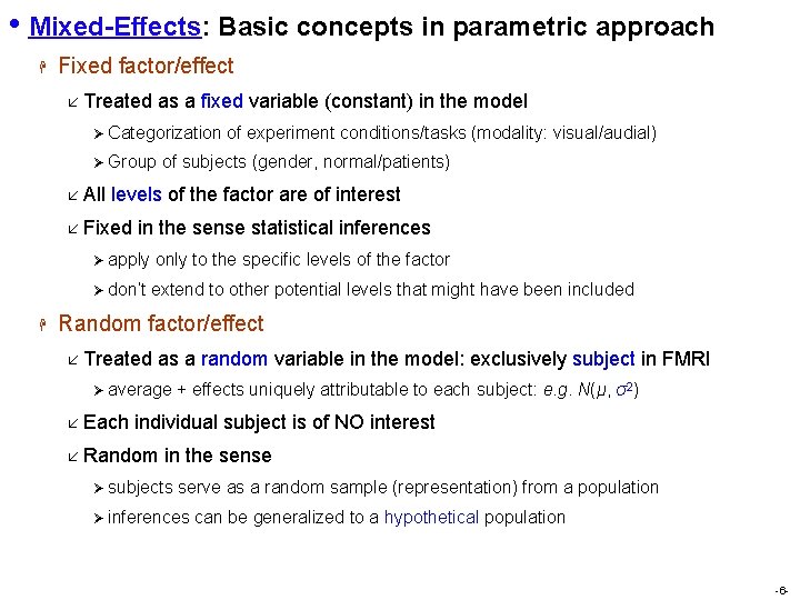
• Mixed-Effects: Basic concepts in parametric approach H Fixed factor/effect å Treated as a fixed variable (constant) in the model Ø Categorization Ø Group å All of subjects (gender, normal/patients) levels of the factor are of interest å Fixed H of experiment conditions/tasks (modality: visual/audial) in the sense statistical inferences Ø apply only to the specific levels of the factor Ø don’t extend to other potential levels that might have been included Random factor/effect å Treated as a random variable in the model: exclusively subject in FMRI Ø average å Each + effects uniquely attributable to each subject: e. g. N(μ, σ2) individual subject is of NO interest å Random in the sense Ø subjects serve as a random sample (representation) from a population Ø inferences can be generalized to a hypothetical population -6 -

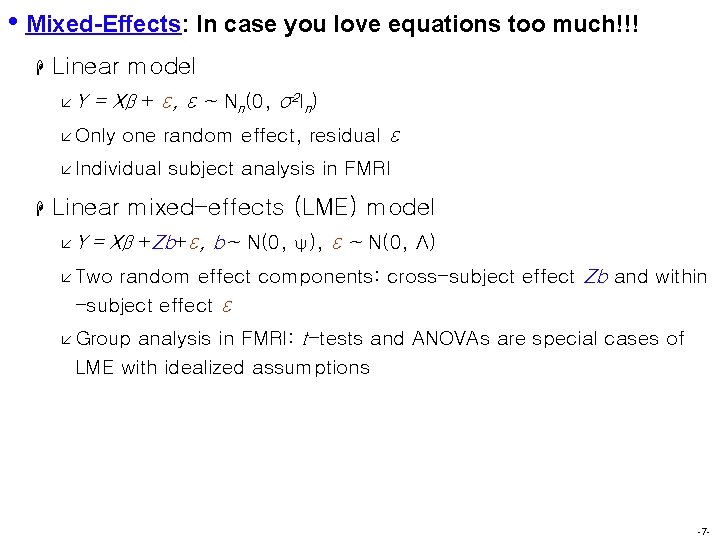
• Mixed-Effects: In case you love equations too much!!! H Linear model åY = Xβ + ε, ε ~ Nn(0, σ2 In) å Only one random effect, residual ε å Individual H subject analysis in FMRI Linear mixed-effects (LME) model åY = Xβ +Zb+ε, b~ N(0, ψ), ε ~ N(0, Λ) random effect components: cross-subject effect Zb and within -subject effect ε å Two analysis in FMRI: t-tests and ANOVAs are special cases of LME with idealized assumptions å Group -7 -

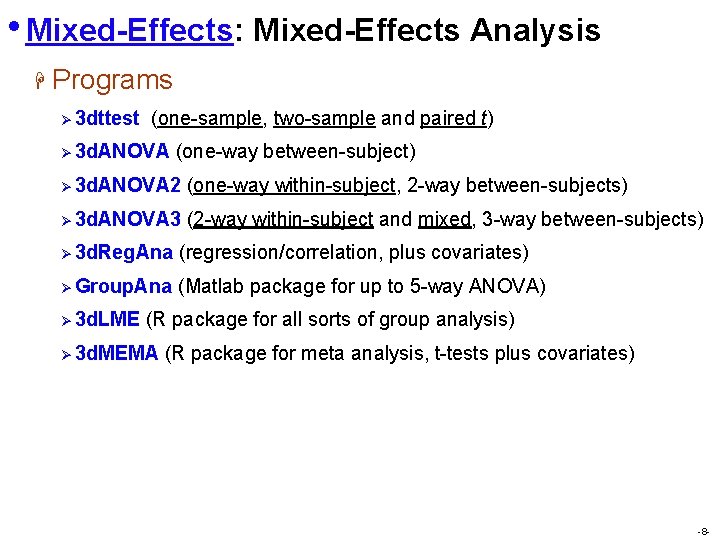
• Mixed-Effects: Mixed-Effects Analysis H Programs Ø 3 dttest (one-sample, two-sample and paired t) Ø 3 d. ANOVA (one-way between-subject) Ø 3 d. ANOVA 2 (one-way within-subject, 2 -way between-subjects) Ø 3 d. ANOVA 3 (2 -way within-subject and mixed, 3 -way between-subjects) Ø 3 d. Reg. Ana (regression/correlation, plus covariates) Ø Group. Ana (Matlab package for up to 5 -way ANOVA) Ø 3 d. LME (R package for all sorts of group analysis) Ø 3 d. MEMA (R package for meta analysis, t-tests plus covariates) -8 -

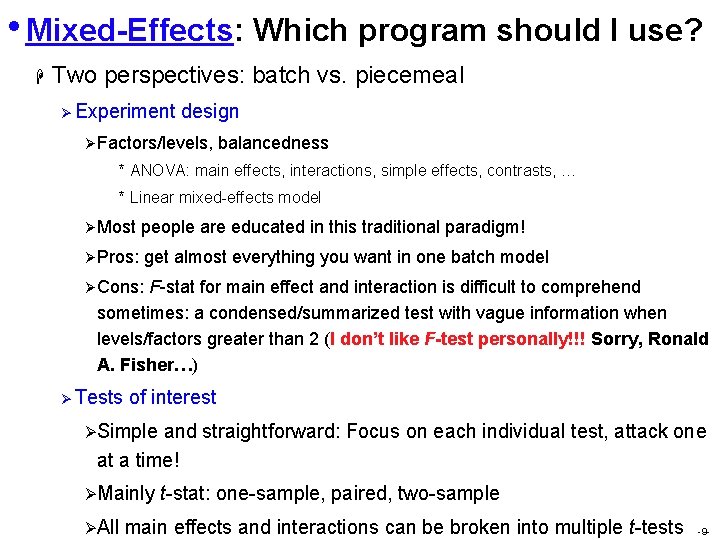
• Mixed-Effects: Which program should I use? H Two perspectives: batch vs. piecemeal Ø Experiment design Ø Factors/levels, balancedness * ANOVA: main effects, interactions, simple effects, contrasts, … * Linear mixed-effects model Ø Most people are educated in this traditional paradigm! Ø Pros: get almost everything you want in one batch model Ø Cons: F-stat for main effect and interaction is difficult to comprehend sometimes: a condensed/summarized test with vague information when levels/factors greater than 2 (I don’t like F-test personally!!! Sorry, Ronald A. Fisher…) Ø Tests of interest ØSimple and straightforward: Focus on each individual test, attack one at a time! ØMainly ØAll t-stat: one-sample, paired, two-sample main effects and interactions can be broken into multiple t-tests -9 -

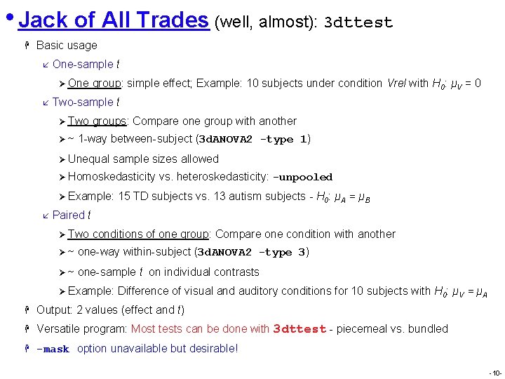
• Jack of All Trades (well, almost): 3 dttest H Basic usage å One-sample t Ø One å group: simple effect; Example: 10 subjects under condition Vrel with H 0: μV = 0 Two-sample t Ø Two Ø~ groups: Compare one group with another 1 -way between-subject (3 d. ANOVA 2 -type 1) Ø Unequal sample sizes allowed Ø Homoskedasticity Ø Example: å vs. heteroskedasticity: -unpooled 15 TD subjects vs. 13 autism subjects - H 0: μA = μB Paired t Ø Two conditions of one group: Compare one condition with another Ø~ one-way within-subject (3 d. ANOVA 2 -type 3) Ø~ one-sample t on individual contrasts Ø Example: Difference of visual and auditory conditions for 10 subjects with H 0: μV = μA H Output: 2 values (effect and t) H Versatile program: Most tests can be done with 3 dttest - piecemeal vs. bundled H -mask option unavailable but desirable! -10 -

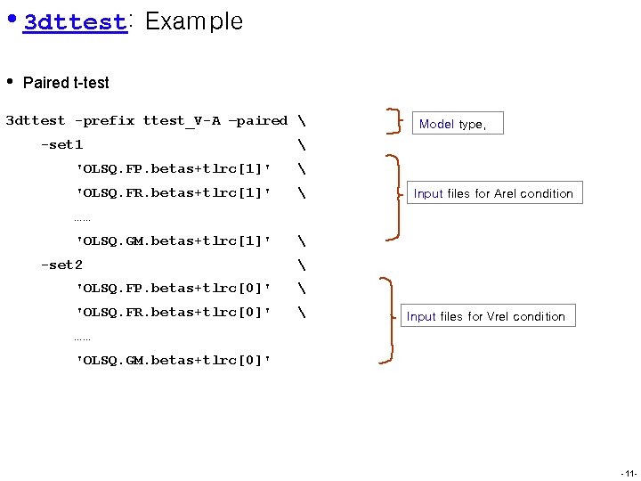
• 3 dttest: Example • Paired t-test 3 dttest -prefix ttest_V-A –paired -set 1 Model type, 'OLSQ. FP. betas+tlrc[1]' 'OLSQ. FR. betas+tlrc[1]' Input files for Arel condition …… 'OLSQ. GM. betas+tlrc[1]' -set 2 'OLSQ. FP. betas+tlrc[0]' 'OLSQ. FR. betas+tlrc[0]' Input files for Vrel condition …… 'OLSQ. GM. betas+tlrc[0]' -11 -

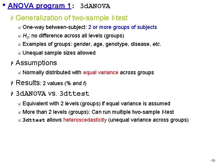
• ANOVA program 1: H Generalization of two-sample t-test å One-way å H 0 : between-subject: 2 or more groups of subjects no difference across all levels (groups) å Examples å Unequal H H of groups: gender, age, genotype, disease, etc. sample sizes allowed Assumptions å Normally H 3 d. ANOVA distributed with equal variance across groups Results: 2 values (% and t) 3 d. ANOVA vs. 3 dttest å Equivalent with 2 levels (groups) if equal variance is assumed å More than 2 levels (groups): Can run multiple two-sample t-test å 3 dttest allows heteroscedasticity (unequal variance across groups) -12 -

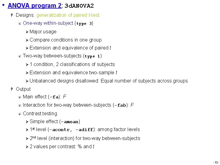
• ANOVA program 2: 3 d. ANOVA 2 H Designs: generalization of paired t-test å One-way within-subject (type 3) Ø Major usage Ø Compare conditions in one group Ø Extension å and equivalence of paired t Two-way between-subjects (type 1) Ø 1 condition, 2 classifications of subjects Ø Extension and equivalence two-sample t Ø Unbalanced H designs disallowed: Equal number of subjects across groups Output å Main effect (-fa): F å Interaction for two-way between-subjects (-fab): F å Contrast testing Ø Simple effect (-amean) Ø 1 st level (-acontr, -adiff): among factor levels Ø 2 nd level (interaction) for two-way between-subjects Ø 2 values per contrast: % and t -13 -

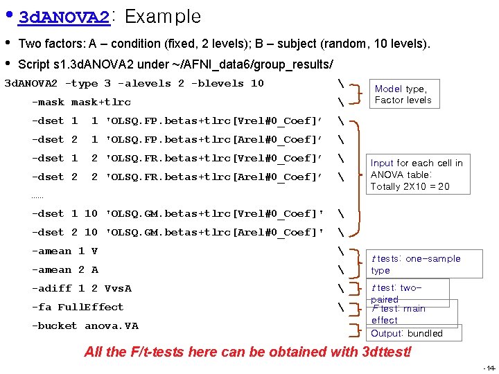
• 3 d. ANOVA 2: Example • • Two factors: A – condition (fixed, 2 levels); B – subject (random, 10 levels). Script s 1. 3 d. ANOVA 2 under ~/AFNI_data 6/group_results/ 3 d. ANOVA 2 -type 3 -alevels 2 -blevels 10 Model type, Factor levels -mask+tlrc -dset 1 1 'OLSQ. FP. betas+tlrc[Vrel#0_Coef]’ -dset 2 1 'OLSQ. FP. betas+tlrc[Arel#0_Coef]’ -dset 1 2 'OLSQ. FR. betas+tlrc[Vrel#0_Coef]’ -dset 2 2 'OLSQ. FR. betas+tlrc[Arel#0_Coef]’ -dset 1 10 'OLSQ. GM. betas+tlrc[Vrel#0_Coef]' -dset 2 10 'OLSQ. GM. betas+tlrc[Arel#0_Coef]' -amean 1 V -amean 2 A type -adiff 1 2 Vvs. A t test: two- -fa Full. Effect …… -bucket anova. VA Input for each cell in ANOVA table: Totally 2 X 10 = 20 t tests: one-sample paired F test: main effect Output: bundled All the F/t-tests here can be obtained with 3 dttest! -14 -

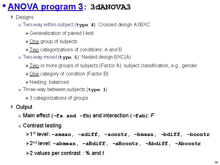
• ANOVA program 3: 3 d. ANOVA 3 H Designs å Two-way within-subject (type 4): Crossed design AXBXC Ø Generalization å Ø One group of subjects Ø Two categorizations of conditions: A and B Two-way mixed (type 5): Nested design BXC(A) Ø Two or more groups of subjects (Factor A): subject classification, e. g. , gender Ø One category of condition (Factor B) Ø Nesting: å balanced Three-way between-subjects (type 1) Ø 3 H of paired t-test categorizations of groups Output å Main effect (-fa and -fb) and interaction (-fab): F å Contrast testing Ø 1 st level: -amean, -adiff, -acontr, -bmean, -bdiff, -bcontr Ø 2 nd level: -abmean, -a. Bdiff, -a. Bcontr, -Abdiff, -Abcontr Ø 2 values per contrast : % and t -15 -

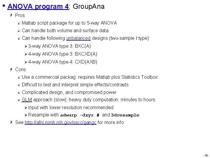
• ANOVA program 4: Group. Ana H H Pros å Matlab script package for up to 5 -way ANOVA å Can handle both volume and surface data å Can handle following unbalanced designs (two-sample t type): Ø 3 -way ANOVA type 3: BXC(A) Ø 4 -way ANOVA type 3: BXCXD(A) Ø 4 -way ANOVA type 4: CXD(AXB) Cons å Use a commercial packag: requires Matlab plus Statistics Toolbox å Difficult to test and interpret simple effects/contrasts å Complicated design, and compromised power å GLM approach (slow): heavy duty computation: minutes to hours Ø Input with lower resolution recommended Ø Resample H with adwarp -dxyz # and 3 dresample See http: //afni. nimh. nih. gov/sscc/gangc for more info -16 -

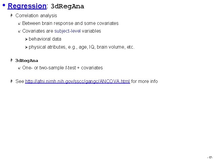
• Regression: 3 d. Reg. Ana H Correlation analysis å Between brain response and some covariates å Covariates are subject-level variables Ø behavioral Ø physical H atributes, e. g. , age, IQ, brain volume, etc. 3 d. Reg. Ana å H data One- or two-sample t-test + covariates See http: //afni. nimh. nih. gov/sscc/gangc/ANCOVA. html for more info -17 -

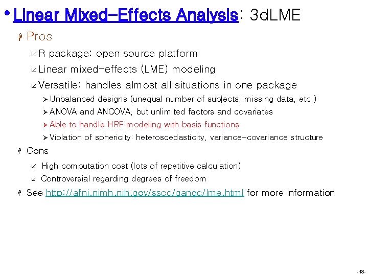
• Linear Mixed-Effects Analysis: 3 d. LME H Pros åR package: open source platform å Linear mixed-effects (LME) modeling å Versatile: handles almost all situations in one package Ø Unbalanced Ø ANOVA Ø Able and ANCOVA, but unlimited factors and covariates to handle HRF modeling with basis functions Ø Violation H H designs (unequal number of subjects, missing data, etc. ) of sphericity: heteroscedasticity, variance-covariance structure Cons å High computation cost (lots of repetitive calculation) å Controversial regarding degrees of freedom See http: //afni. nimh. nih. gov/sscc/gangc/lme. html for more information -18 -

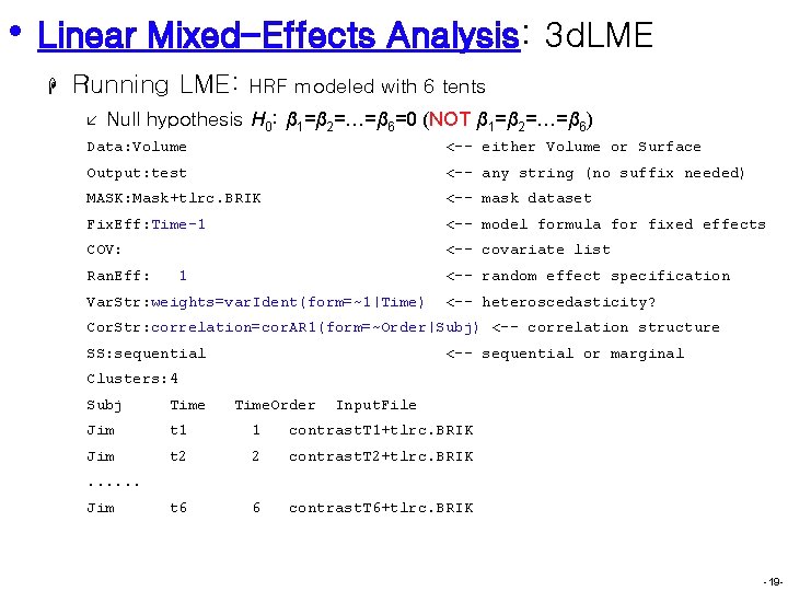
• Linear Mixed-Effects Analysis: 3 d. LME H Running LME: å HRF modeled with 6 tents Null hypothesis H 0: β 1=β 2=…=β 6=0 (NOT β 1=β 2=…=β 6) Data: Volume <-- either Volume or Surface Output: test <-- any string (no suffix needed) MASK: Mask+tlrc. BRIK <-- mask dataset Fix. Eff: Time-1 <-- model formula for fixed effects COV: <-- covariate list Ran. Eff: 1 <-- random effect specification Var. Str: weights=var. Ident(form=~1|Time) <-- heteroscedasticity? Cor. Str: correlation=cor. AR 1(form=~Order|Subj) <-- correlation structure SS: sequential <-- sequential or marginal Clusters: 4 Subj Time. Order Input. File Jim t 1 1 contrast. T 1+tlrc. BRIK Jim t 2 2 contrast. T 2+tlrc. BRIK t 6 6 contrast. T 6+tlrc. BRIK . . . Jim -19 -

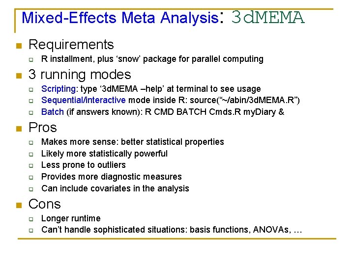
Mixed-Effects Meta Analysis: n Requirements q n q q Scripting: type ‘ 3 d. MEMA –help’ at terminal to see usage Sequential/interactive mode inside R: source(“~/abin/3 d. MEMA. R”) Batch (if answers known): R CMD BATCH Cmds. R my. Diary & Pros q q q n R installment, plus ‘snow’ package for parallel computing 3 running modes q n 3 d. MEMA Makes more sense: better statistical properties Likely more statistically powerful Less prone to outliers Provides more diagnostic measures Can include covariates in the analysis Cons q q Longer runtime Can’t handle sophisticated situations: basis functions, ANOVAs, …

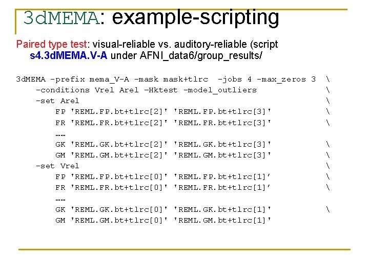
3 d. MEMA: example-scripting Paired type test: visual-reliable vs. auditory-reliable (script s 4. 3 d. MEMA. V-A under AFNI_data 6/group_results/ 3 d. MEMA -prefix mema_V-A -mask+tlrc -jobs 4 -max_zeros 3 -conditions Vrel Arel –Hktest -model_outliers -set Arel FP 'REML. FP. bt+tlrc[2]' 'REML. FP. bt+tlrc[3]' FR 'REML. FR. bt+tlrc[2]' 'REML. FR. bt+tlrc[3]' …… GK 'REML. GK. bt+tlrc[2]' 'REML. GK. bt+tlrc[3]' GM 'REML. GM. bt+tlrc[2]' 'REML. GM. bt+tlrc[3]' -set Vrel FP 'REML. FP. bt+tlrc[0]' 'REML. FP. bt+tlrc[1]’ FR 'REML. FR. bt+tlrc[0]' 'REML. FR. bt+tlrc[1]’ …… GK 'REML. GK. bt+tlrc[0]' 'REML. GK. bt+tlrc[1]' GM 'REML. GM. bt+tlrc[0]' 'REML. GM. bt+tlrc[1]'

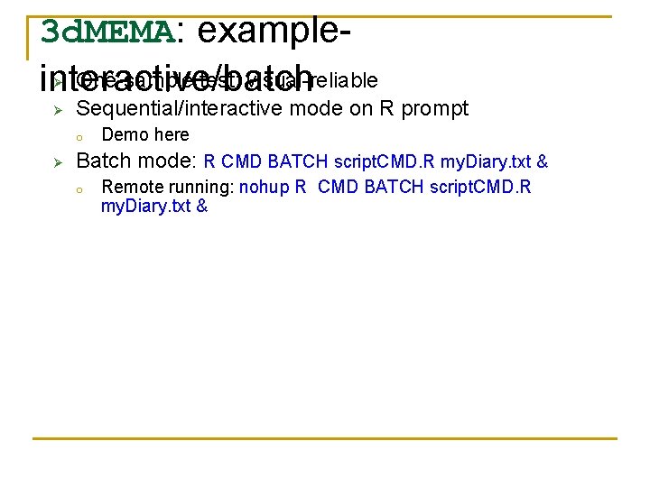
3 d. MEMA: example. One-sample test: visual-reliable interactive/batch Ø Ø Sequential/interactive mode on R prompt o Ø Demo here Batch mode: R CMD BATCH script. CMD. R my. Diary. txt & o Remote running: nohup R CMD BATCH script. CMD. R my. Diary. txt &

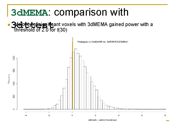
n 3 d. MEMA: comparison with Majority of significant voxels with 3 d. MEMA gained power with a 3 dttest threshold of 2. 0 for t(30)

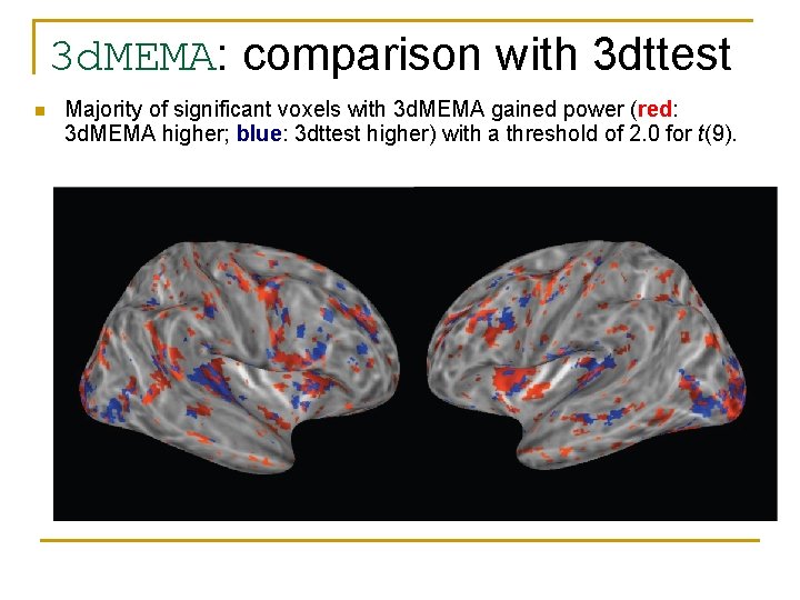
3 d. MEMA: comparison with 3 dttest n Majority of significant voxels with 3 d. MEMA gained power (red: 3 d. MEMA higher; blue: 3 dttest higher) with a threshold of 2. 0 for t(9).

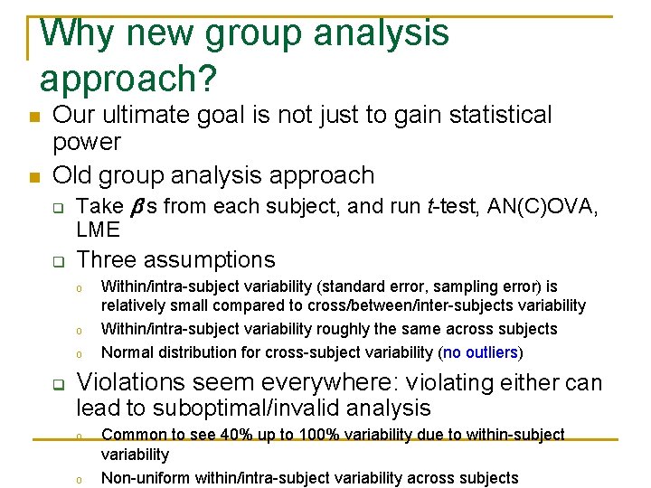
Why new group analysis approach? n n Our ultimate goal is not just to gain statistical power Old group analysis approach q q Take ’s from each subject, and run t-test, AN(C)OVA, LME Three assumptions o o o q Within/intra-subject variability (standard error, sampling error) is relatively small compared to cross/between/inter-subjects variability Within/intra-subject variability roughly the same across subjects Normal distribution for cross-subject variability (no outliers) Violations seem everywhere: violating either can lead to suboptimal/invalid analysis o o Common to see 40% up to 100% variability due to within-subject variability Non-uniform within/intra-subject variability across subjects

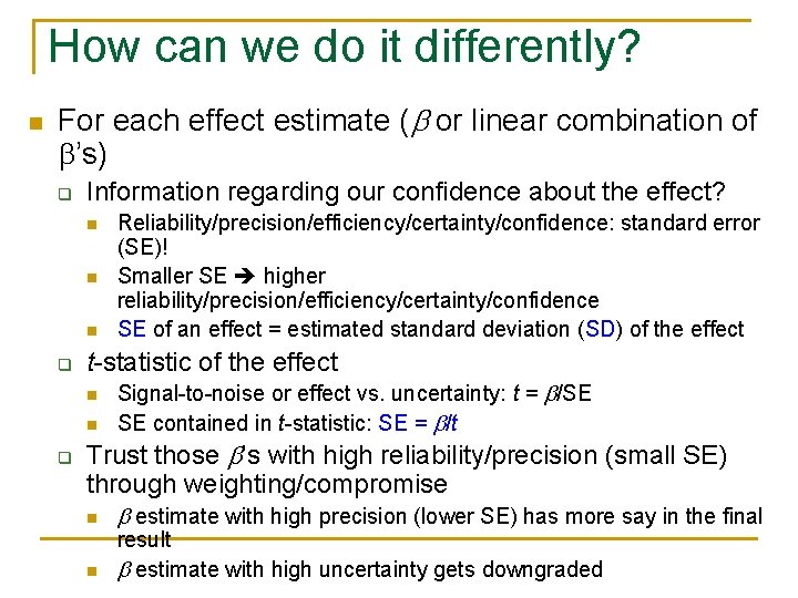
How can we do it differently? n For each effect estimate ( or linear combination of ’s) q Information regarding our confidence about the effect? n n n q t-statistic of the effect n n q Reliability/precision/efficiency/certainty/confidence: standard error (SE)! Smaller SE higher reliability/precision/efficiency/certainty/confidence SE of an effect = estimated standard deviation (SD) of the effect Signal-to-noise or effect vs. uncertainty: t = /SE SE contained in t-statistic: SE = /t Trust those ’s with high reliability/precision (small SE) through weighting/compromise n n estimate with high precision (lower SE) has more say in the final result estimate with high uncertainty gets downgraded

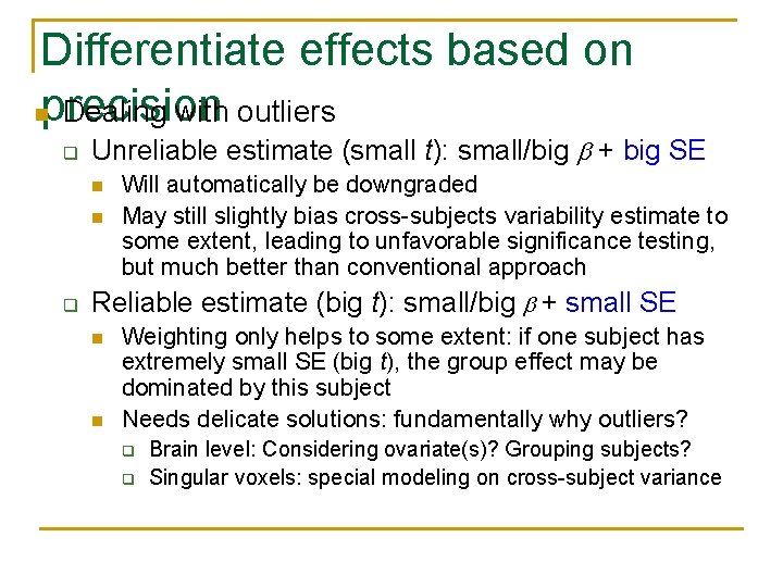
Differentiate effects based on nprecision Dealing with outliers q Unreliable estimate (small t): small/big + big SE n n q Will automatically be downgraded May still slightly bias cross-subjects variability estimate to some extent, leading to unfavorable significance testing, but much better than conventional approach Reliable estimate (big t): small/big + small SE n n Weighting only helps to some extent: if one subject has extremely small SE (big t), the group effect may be dominated by this subject Needs delicate solutions: fundamentally why outliers? q q Brain level: Considering ovariate(s)? Grouping subjects? Singular voxels: special modeling on cross-subject variance

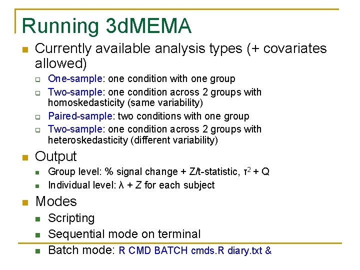
Running 3 d. MEMA n Currently available analysis types (+ covariates allowed) q q n Output n n n One-sample: one condition with one group Two-sample: one condition across 2 groups with homoskedasticity (same variability) Paired-sample: two conditions with one group Two-sample: one condition across 2 groups with heteroskedasticity (different variability) Group level: % signal change + Z/t-statistic, τ2 + Q Individual level: λ + Z for each subject Modes n n n Scripting Sequential mode on terminal Batch mode: R CMD BATCH cmds. R diary. txt &

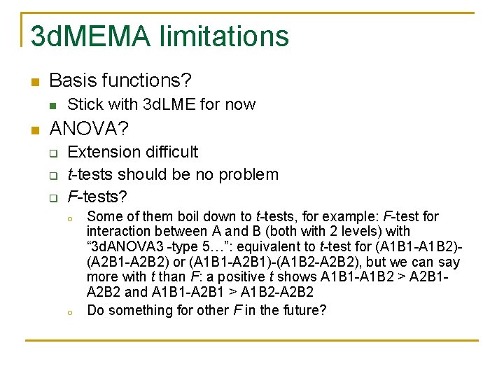
3 d. MEMA limitations n Basis functions? n n Stick with 3 d. LME for now ANOVA? q q q Extension difficult t-tests should be no problem F-tests? o o Some of them boil down to t-tests, for example: F-test for interaction between A and B (both with 2 levels) with “ 3 d. ANOVA 3 -type 5…”: equivalent to t-test for (A 1 B 1 -A 1 B 2)(A 2 B 1 -A 2 B 2) or (A 1 B 1 -A 2 B 1)-(A 1 B 2 -A 2 B 2), but we can say more with t than F: a positive t shows A 1 B 1 -A 1 B 2 > A 2 B 1 A 2 B 2 and A 1 B 1 -A 2 B 1 > A 1 B 2 -A 2 B 2 Do something for other F in the future?

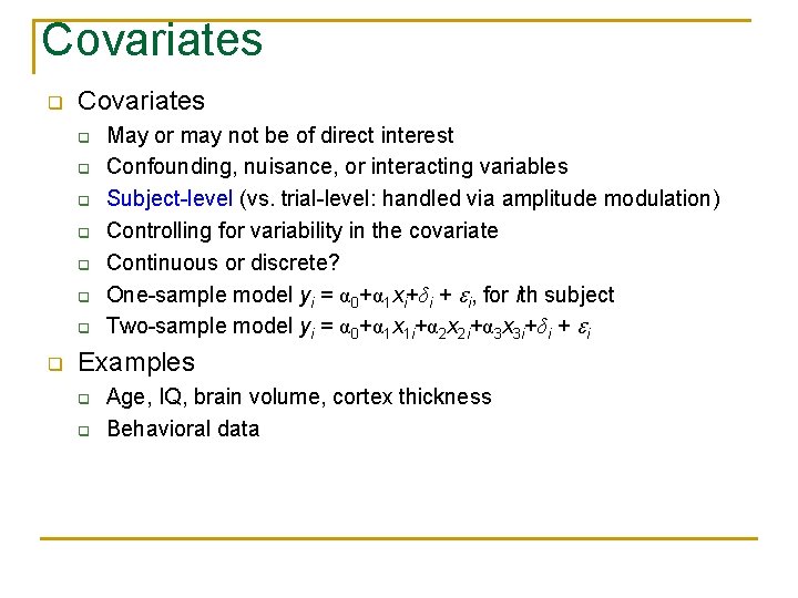
Covariates q q q q q May or may not be of direct interest Confounding, nuisance, or interacting variables Subject-level (vs. trial-level: handled via amplitude modulation) Controlling for variability in the covariate Continuous or discrete? One-sample model yi = α 0+α 1 xi+δi + i, for ith subject Two-sample model yi = α 0+α 1 x 1 i+α 2 x 2 i+α 3 x 3 i+δi + i Examples q q Age, IQ, brain volume, cortex thickness Behavioral data

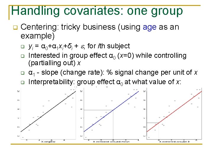
Handling covariates: one group q Centering: tricky business (using age as an example) q q yi = α 0+α 1 xi+δi + , for ith subject Interested in group effect α 0 (x=0) while controlling (partialling out) x α 1 - slope (change rate): % signal change per unit of x Interpretability: group effect α 0 at what value of x: mean or any other value?

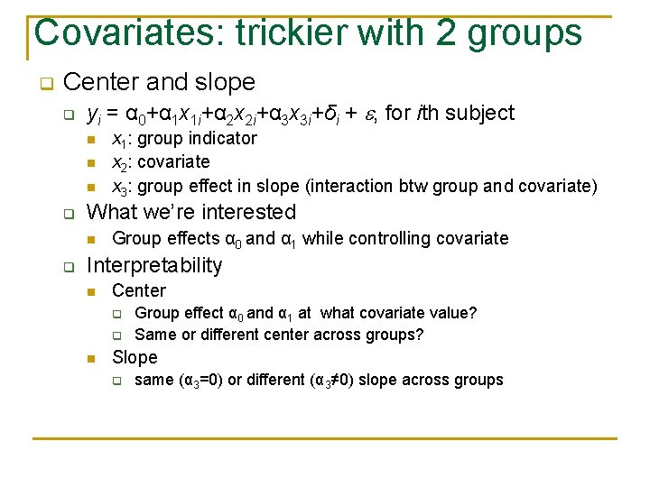
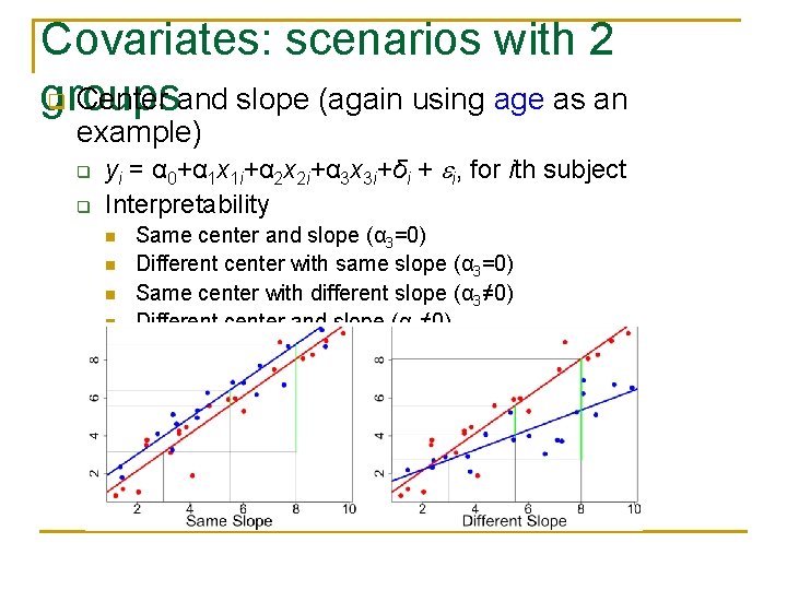
Covariates: trickier with 2 groups q Center and slope q yi = α 0+α 1 x 1 i+α 2 x 2 i+α 3 x 3 i+δi + , for ith subject n n n q What we’re interested n q x 1: group indicator x 2: covariate x 3: group effect in slope (interaction btw group and covariate) Group effects α 0 and α 1 while controlling covariate Interpretability n Center q q n Group effect α 0 and α 1 at what covariate value? Same or different center across groups? Slope q same (α 3=0) or different (α 3≠ 0) slope across groups

Covariates: scenarios with 2 q Center and slope (again using age as an groups example) q q yi = α 0+α 1 x 1 i+α 2 x 2 i+α 3 x 3 i+δi + i, for ith subject Interpretability n n Same center and slope (α 3=0) Different center with same slope (α 3=0) Same center with different slope (α 3≠ 0) Different center and slope (α 3≠ 0)

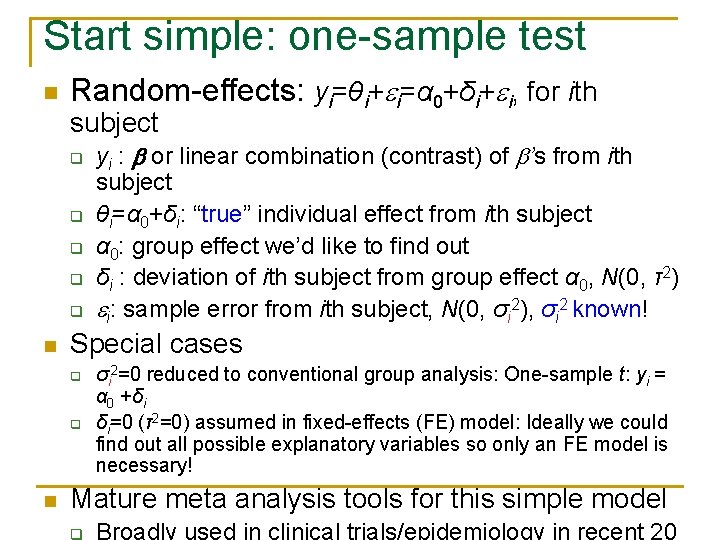
Start simple: one-sample test n Random-effects: yi=θi+ i=α 0+δi+ i, for ith subject q q q n Special cases q q n yi : or linear combination (contrast) of ’s from ith subject θi=α 0+δi: “true” individual effect from ith subject α 0: group effect we’d like to find out δi : deviation of ith subject from group effect α 0, N(0, τ2) i: sample error from ith subject, N(0, σi 2), σi 2 known! σi 2=0 reduced to conventional group analysis: One-sample t: yi = α 0 +δi δi=0 (τ2=0) assumed in fixed-effects (FE) model: Ideally we could find out all possible explanatory variables so only an FE model is necessary! Mature meta analysis tools for this simple model

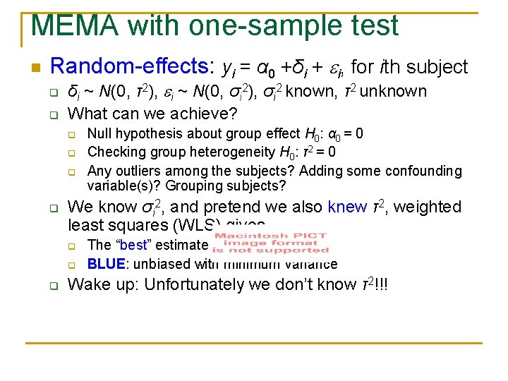
MEMA with one-sample test n Random-effects: yi = α 0 +δi + i, for ith subject q q δi ~ N(0, τ2), i ~ N(0, σi 2), σi 2 known, τ2 unknown What can we achieve? q q We know σi 2, and pretend we also knew τ2, weighted least squares (WLS) gives q q q Null hypothesis about group effect H 0: α 0 = 0 Checking group heterogeneity H 0: τ2 = 0 Any outliers among the subjects? Adding some confounding variable(s)? Grouping subjects? The “best” estimate BLUE: unbiased with minimum variance Wake up: Unfortunately we don’t know τ2!!!

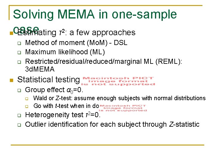
Solving MEMA in one-sample ncase Estimating τ2: a few approaches q q q n Method of moment (Mo. M) - DSL Maximum likelihood (ML) Restricted/residual/reduced/marginal ML (REML): 3 d. MEMA Statistical testing q Group effect α 0=0: q q Wald or Z-test: assume enough subjects with normal distributions Go with t-test when in doubt Heterogeneity test τ2=0: Outlier identification for each subject through Z-statistic

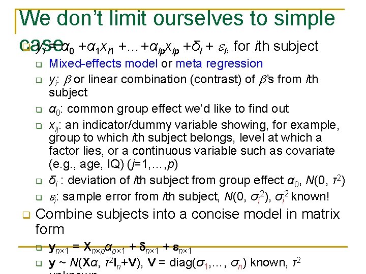
We don’t limit ourselves to simple q yi = α 0 +α 1 xi 1 +…+αipxip +δi + i, for ith subject case q q q q Mixed-effects model or meta regression yi: or linear combination (contrast) of ’s from ith subject α 0: common group effect we’d like to find out xij: an indicator/dummy variable showing, for example, group to which ith subject belongs, level at which a factor lies, or a continuous variable such as covariate (e. g. , age, IQ) (j=1, …, p) δi : deviation of ith subject from group effect α 0, N(0, τ2) i: sample error from ith subject, N(0, σi 2), σi 2 known! Combine subjects into a concise model in matrix form q q yn× 1 = Xn×pαp× 1 + n× 1 y ~ N(Xα, τ2 In+V), V = diag(σ1, …, σn) known, τ2

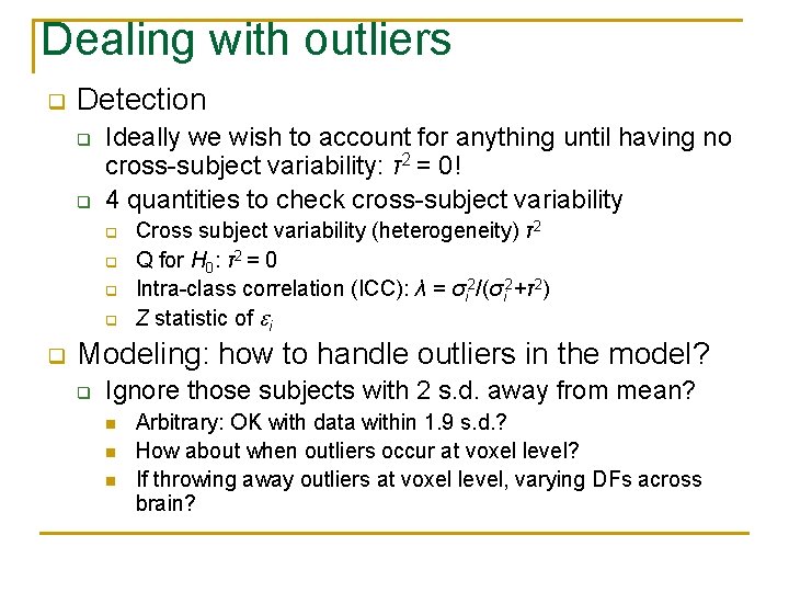
Dealing with outliers q Detection q q Ideally we wish to account for anything until having no cross-subject variability: τ2 = 0! 4 quantities to check cross-subject variability q q q Cross subject variability (heterogeneity) τ2 Q for H 0: τ2 = 0 Intra-class correlation (ICC): λ = σi 2/(σi 2+τ2) Z statistic of i Modeling: how to handle outliers in the model? q Ignore those subjects with 2 s. d. away from mean? n n n Arbitrary: OK with data within 1. 9 s. d. ? How about when outliers occur at voxel level? If throwing away outliers at voxel level, varying DFs across brain?

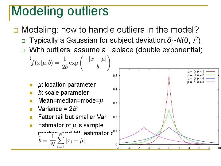
Modeling outliers q Modeling: how to handle outliers in the model? q q Typically a Gaussian for subject deviation: δi~N(0, τ2) With outliers, assume a Laplace (double exponential) distribution n n n μ: location parameter b: scale parameter Mean=median=mode=μ Variance = 2 b 2 Fatter tail but smaller Var Estimator of μ is sample median, and ML estimator of b

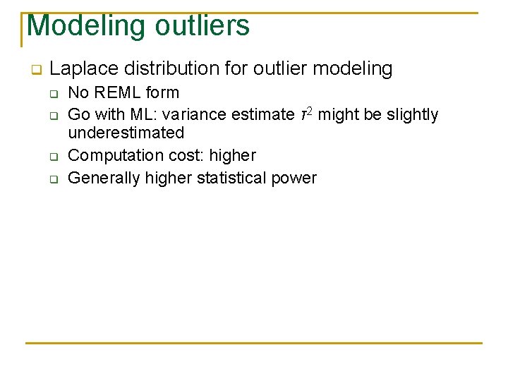
Modeling outliers q Laplace distribution for outlier modeling q q No REML form Go with ML: variance estimate τ2 might be slightly underestimated Computation cost: higher Generally higher statistical power

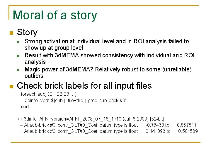
Moral of a story n Story n n Strong activation at individual level and in ROI analysis failed to show up at group level Result with 3 d. MEMA showed consistency with individual and ROI analysis Magic power of 3 d. MEMA? Relatively robust to some (unreliable) outliers Check brick labels for all input files foreach subj (S 1 S 2 S 3 …) 3 dinfo -verb ${subj}_file+tlrc | grep 'sub-brick #0’ end ++ 3 dinfo: AFNI version=AFNI_2008_07_18_1710 (Jul 8 2009) [32 -bit] -- At sub-brick #0 ’contr_GLT#0_Coef' datum type is float: -0. 78438 to -- At sub-brick #0 ’contr_GLT#0_Coef' datum type is float: -0. 444093 to … 0. 867817 0. 501589

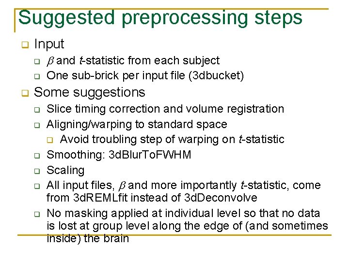
Suggested preprocessing steps q q Input q and t-statistic from each subject q One sub-brick per input file (3 dbucket) Some suggestions q q q Slice timing correction and volume registration Aligning/warping to standard space q Avoid troubling step of warping on t-statistic Smoothing: 3 d. Blur. To. FWHM Scaling All input files, and more importantly t-statistic, come from 3 d. REMLfit instead of 3 d. Deconvolve No masking applied at individual level so that no data is lost at group level along the edge of (and sometimes inside) the brain

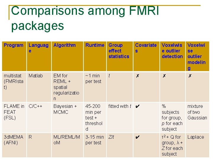
Comparisons among FMRI packages Program Languag e Algorithm Runtime Group effect statistics Covariate s Voxelwi e outlier se detection outlier modelin g multistat (FMRIsta t) Matlab EM for REML + spatial regularizatio n ~1 min per test t ✗ ✗ FLAME in C/C++ FEAT (FSL) Bayesian + MCMC 45 -200 min per test + threshol d fitted with t ✔ 3 d. MEMA (AFNI) ML/REML/M o. M 3 -15 min Z/t per test R ✔ ✗ % mixture subjects of two for group, Gaussian p for each subject τ2 + Q for Laplace group, λ + Z for each subject

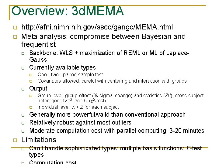
Overview: 3 d. MEMA q q http: //afni. nimh. nih. gov/sscc/gangc/MEMA. html Meta analysis: compromise between Bayesian and frequentist q q Backbone: WLS + maximization of REML or ML of Laplace. Gauss Currently available types q q q Output q q q One-, two-, paired-sample test Covariates allowed: careful with centering and interaction with groups Group level: group effect (% sigmal change) and statistics (Z/t), cross-subject heterogeneity τ2 and Q (χ2 -test) Individual level: λ + Z for each subject Generally more powerful/valid than conventional approach Relatively robust against most outliers Moderate computation cost with parallel computing: 3 -20 minutes Limitations q Can’t handle sophisticated types: multiple basis functions; F-test types