ES 240 Scientific and Engineering Computation Chapter 6

ES 240: Scientific and Engineering Computation. Chapter 6 Uchechukwu Ofoegbu Temple University Chapter 6: Roots: Open Methods

ES 240: Scientific and Engineering Computation. Chapter 6 Open Methods § Open methods versus bracketing methods: – Open methods require only a single starting value or two starting values that do not necessarily bracket a root. – Open methods may diverge as the computation progresses – When open methods do converge, they usually do so much faster than bracketing methods.

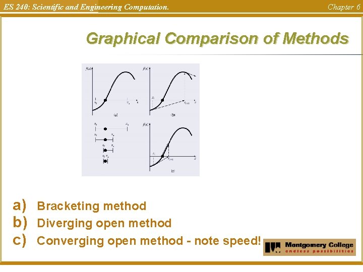
ES 240: Scientific and Engineering Computation. Chapter 6 Graphical Comparison of Methods a) b) c) Bracketing method Diverging open method Converging open method - note speed!

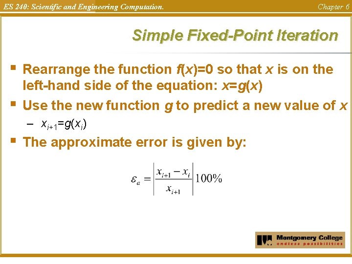
ES 240: Scientific and Engineering Computation. Chapter 6 Simple Fixed-Point Iteration § § § Rearrange the function f(x)=0 so that x is on the left-hand side of the equation: x=g(x) Use the new function g to predict a new value of x – xi+1=g(xi) The approximate error is given by:

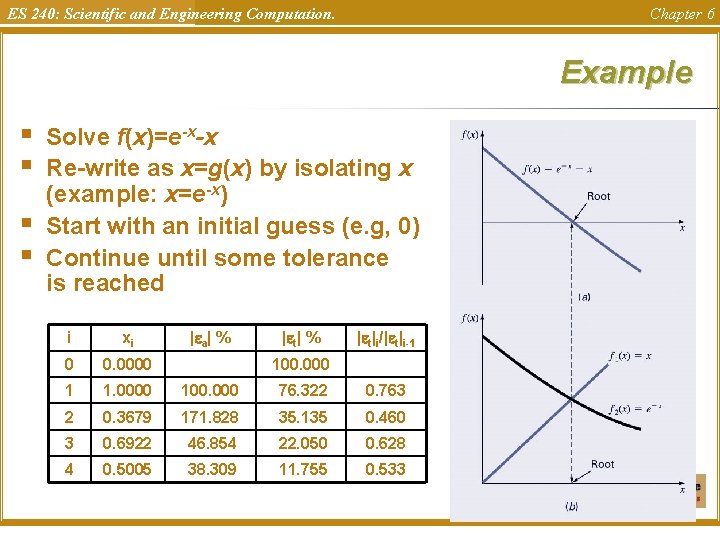
ES 240: Scientific and Engineering Computation. Chapter 6 Example § § Solve f(x)=e-x-x Re-write as x=g(x) by isolating x (example: x=e-x) Start with an initial guess (e. g, 0) Continue until some tolerance is reached i xi | a| % | t|i/| t|i-1 0 0. 0000 1 1. 0000 100. 000 76. 322 0. 763 2 0. 3679 171. 828 35. 135 0. 460 3 0. 6922 46. 854 22. 050 0. 628 4 0. 5005 38. 309 11. 755 0. 533 100. 000

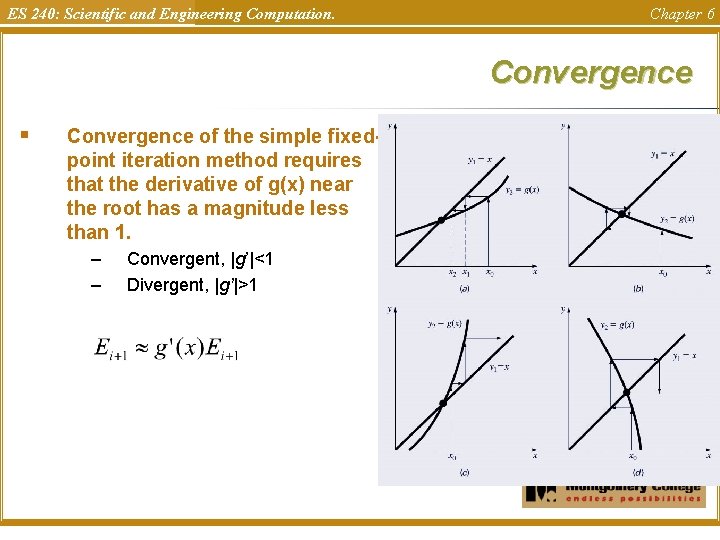
ES 240: Scientific and Engineering Computation. Chapter 6 Convergence § Convergence of the simple fixedpoint iteration method requires that the derivative of g(x) near the root has a magnitude less than 1. – – Convergent, |g’|<1 Divergent, |g’|>1

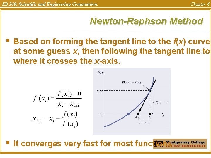
ES 240: Scientific and Engineering Computation. Chapter 6 Newton-Raphson Method § Based on forming the tangent line to the f(x) curve at some guess x, then following the tangent line to where it crosses the x-axis. § It converges very fast for most functions

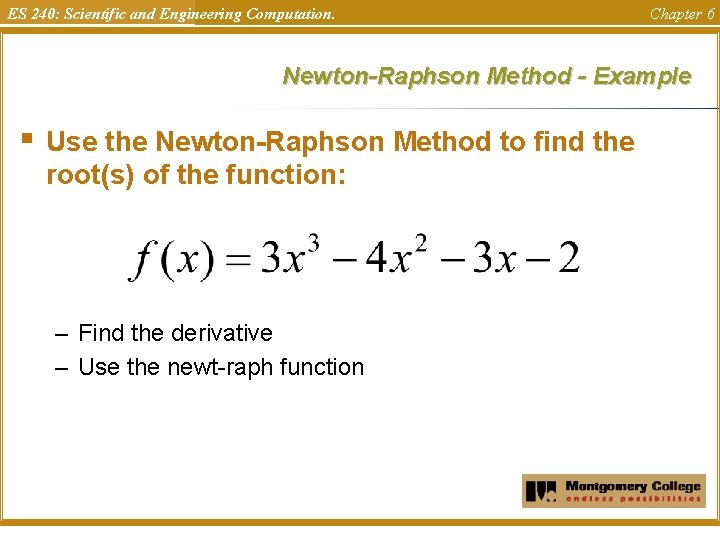
ES 240: Scientific and Engineering Computation. Chapter 6 Newton-Raphson Method - Example § Use the Newton-Raphson Method to find the root(s) of the function: – Find the derivative – Use the newt-raph function

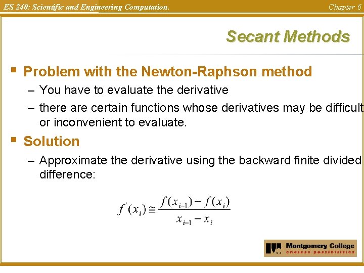
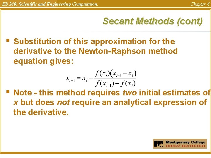
ES 240: Scientific and Engineering Computation. Chapter 6 Secant Methods § Problem with the Newton-Raphson method – You have to evaluate the derivative – there are certain functions whose derivatives may be difficult or inconvenient to evaluate. § Solution – Approximate the derivative using the backward finite divided difference:

ES 240: Scientific and Engineering Computation. Chapter 6 Secant Methods (cont) § Substitution of this approximation for the derivative to the Newton-Raphson method equation gives: § Note - this method requires two initial estimates of x but does not require an analytical expression of the derivative.

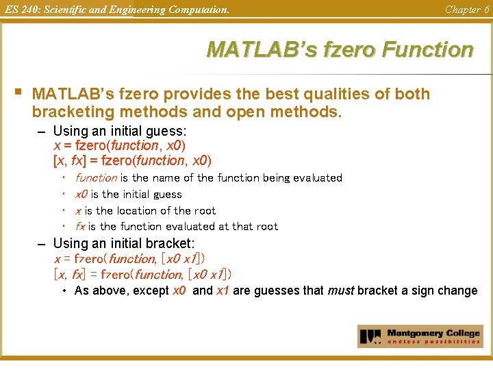
ES 240: Scientific and Engineering Computation. Chapter 6 MATLAB’s fzero Function § MATLAB’s fzero provides the best qualities of both bracketing methods and open methods. – Using an initial guess: x = fzero(function, x 0) [x, fx] = fzero(function, x 0) function is the name of the function being evaluated x 0 is the initial guess x is the location of the root fx is the function evaluated at that root – Using an initial bracket: x = fzero(function, [x 0 x 1]) [x, fx] = fzero(function, [x 0 x 1]) • As above, except x 0 and x 1 are guesses that must bracket a sign change • •

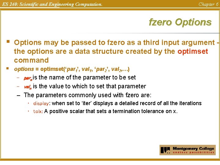
ES 240: Scientific and Engineering Computation. Chapter 6 fzero Options § Options may be passed to fzero as a third input argument the options are a data structure created by the optimset command § options = optimset(‘par 1’, val 1, ‘par 2’, val 2, …) – parn is the name of the parameter to be set – valn is the value to which to set that parameter – The parameters commonly used with fzero are: • display: when set to ‘iter’ displays a detailed record of all the iterations • tolx: A positive scalar that sets a termination tolerance on x.

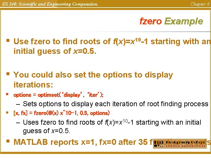
ES 240: Scientific and Engineering Computation. Chapter 6 fzero Example § Use fzero to find roots of f(x)=x 10 -1 starting with an initial guess of x=0. 5. § You could also set the options to display iterations: § options = optimset(‘display’, ‘iter’); – Sets options to display each iteration of root finding process § [x, fx] = fzero(@(x) x^10 -1, 0. 5, options) – Uses fzero to find roots of f(x)=x 10 -1 starting with an initial guess of x=0. 5. § MATLAB reports x=1, fx=0 after 35 function counts

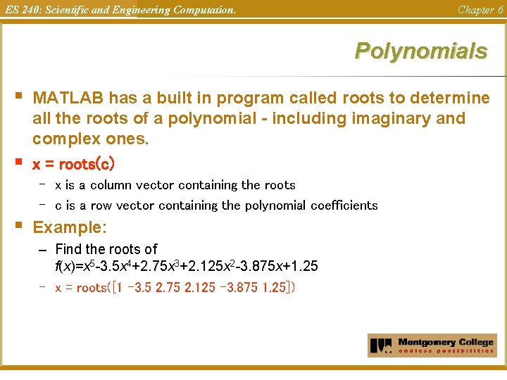
ES 240: Scientific and Engineering Computation. Chapter 6 Polynomials § § MATLAB has a built in program called roots to determine all the roots of a polynomial - including imaginary and complex ones. x = roots(c) – x is a column vector containing the roots – c is a row vector containing the polynomial coefficients § Example: – Find the roots of f(x)=x 5 -3. 5 x 4+2. 75 x 3+2. 125 x 2 -3. 875 x+1. 25 – x = roots([1 -3. 5 2. 75 2. 125 -3. 875 1. 25])

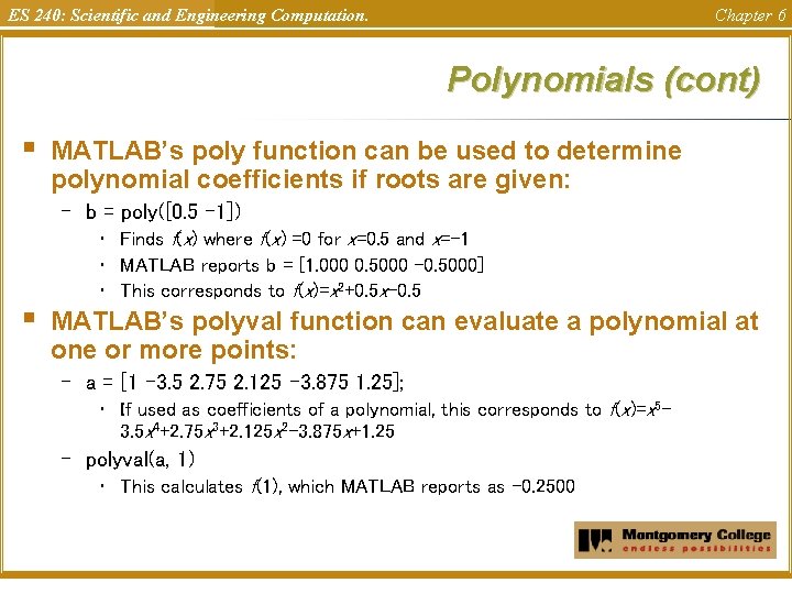
ES 240: Scientific and Engineering Computation. Chapter 6 Polynomials (cont) § MATLAB’s poly function can be used to determine polynomial coefficients if roots are given: – b = poly([0. 5 -1]) § • Finds f(x) where f(x) =0 for x=0. 5 and x=-1 • MATLAB reports b = [1. 000 0. 5000 -0. 5000] • This corresponds to f(x)=x 2+0. 5 x-0. 5 MATLAB’s polyval function can evaluate a polynomial at one or more points: – a = [1 -3. 5 2. 75 2. 125 -3. 875 1. 25]; • If used as coefficients of a polynomial, this corresponds to f(x)=x 53. 5 x 4+2. 75 x 3+2. 125 x 2 -3. 875 x+1. 25 – polyval(a, 1) • This calculates f(1), which MATLAB reports as -0. 2500

ES 240: Scientific and Engineering Computation. Chapter 6 Lab § Ex 6. 4 a&b – Do this step by step in Matlab