ENIAC University of Pennsylvania 1945 ENIAC museum First

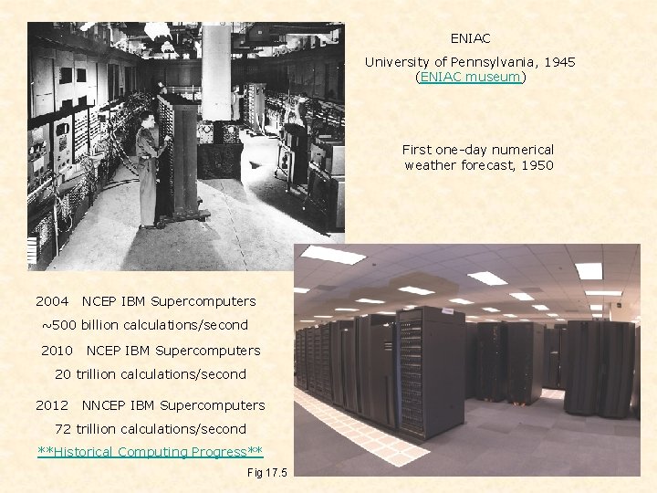
ENIAC University of Pennsylvania, 1945 (ENIAC museum) First one-day numerical weather forecast, 1950 2004 NCEP IBM Supercomputers ~500 billion calculations/second 2010 NCEP IBM Supercomputers 20 trillion calculations/second 2012 NNCEP IBM Supercomputers 72 trillion calculations/second **Historical Computing Progress** Fig 17. 5

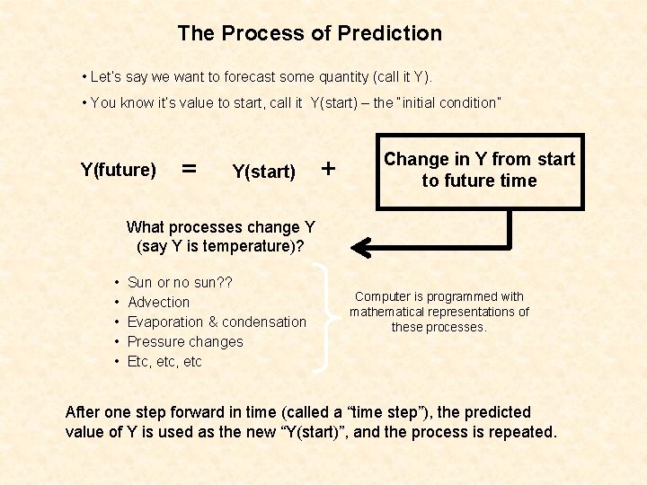
The Process of Prediction • Let’s say we want to forecast some quantity (call it Y). • You know it’s value to start, call it Y(start) – the “initial condition” Y(future) = Y(start) + Change in Y from start to future time What processes change Y (say Y is temperature)? • • • Sun or no sun? ? Advection Evaporation & condensation Pressure changes Etc, etc Computer is programmed with mathematical representations of these processes. After one step forward in time (called a “time step”), the predicted value of Y is used as the new “Y(start)”, and the process is repeated.

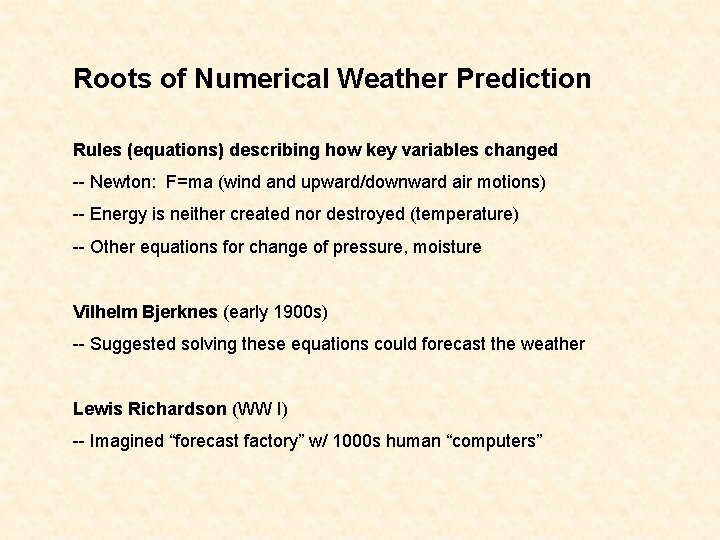
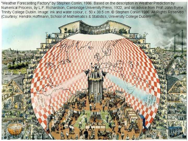
Roots of Numerical Weather Prediction Rules (equations) describing how key variables changed -- Newton: F=ma (wind and upward/downward air motions) -- Energy is neither created nor destroyed (temperature) -- Other equations for change of pressure, moisture Vilhelm Bjerknes (early 1900 s) -- Suggested solving these equations could forecast the weather Lewis Richardson (WW I) -- Imagined “forecast factory” w/ 1000 s human “computers”

“Weather Forecasting Factory” by Stephen Conlin, 1986. Based on the description in Weather Prediction by Numerical Process, by L. F. Richardson, Cambridge University Press, 1922, and on advice from Prof. John Byrne, Trinity College Dublin. Image: ink and water colour, c. 50 x 38. 5 cm. © Stephen Conlin 1986. All Rights Reserved ´. (Courtesy: Hendrik Hoffmann, School of Mathematics & Statistics, University College Dublin)

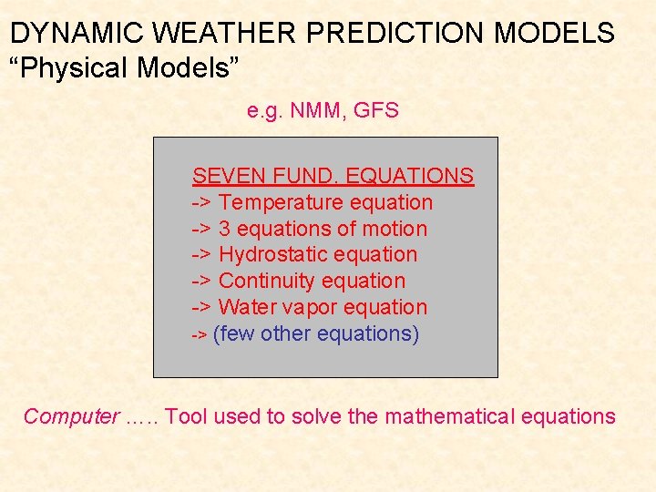
DYNAMIC WEATHER PREDICTION MODELS “Physical Models” e. g. NMM, GFS SEVEN FUND. EQUATIONS -> Temperature equation -> 3 equations of motion -> Hydrostatic equation -> Continuity equation -> Water vapor equation -> (few other equations) Computer …. . Tool used to solve the mathematical equations

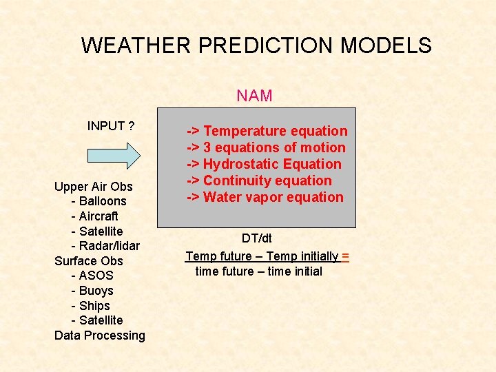
WEATHER PREDICTION MODELS NAM INPUT ? Upper Air Obs - Balloons - Aircraft - Satellite - Radar/lidar Surface Obs - ASOS - Buoys - Ships - Satellite Data Processing -> Temperature equation -> 3 equations of motion -> Hydrostatic Equation -> Continuity equation -> Water vapor equation DT/dt Temp future – Temp initially = time future – time initial

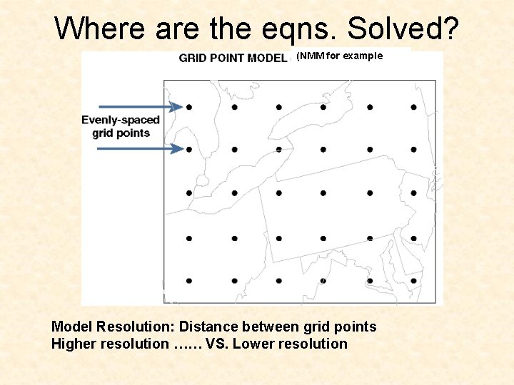
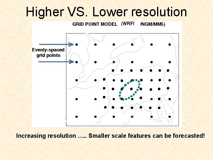
Where are the eqns. Solved? (NMM for example Model Resolution: Distance between grid points Higher resolution …… VS. Lower resolution

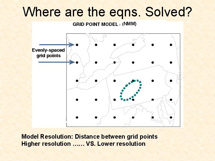
Where are the eqns. Solved? (NMM) Model Resolution: Distance between grid points Higher resolution …… VS. Lower resolution

Higher VS. Lower resolution (WRF/ Increasing resolution …. . Smaller scale features can be forecasted!

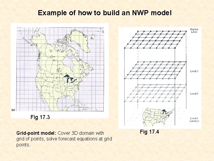
Example of how to build an NWP model Fig 17. 3 Grid-point model: Cover 3 D domain with grid of points, solve forecast equations at grid points. Fig 17. 4

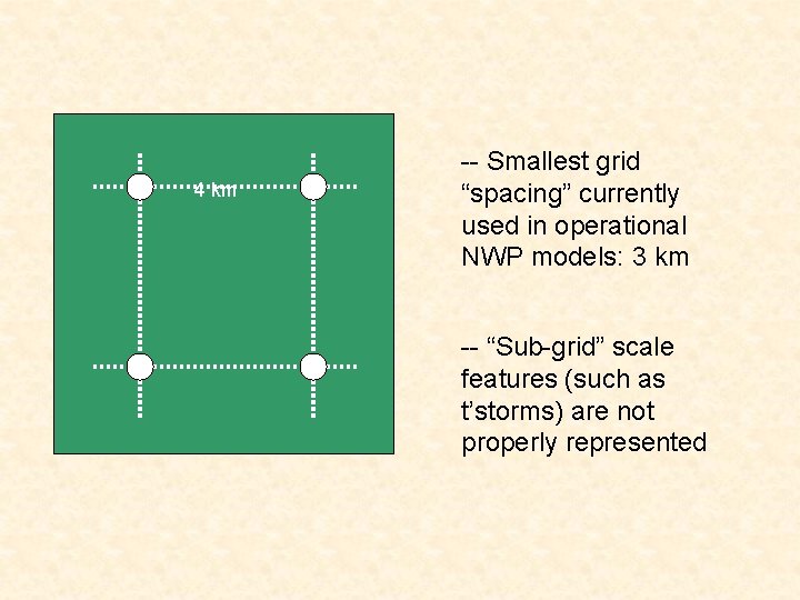
4 km -- Smallest grid “spacing” currently used in operational NWP models: 3 km -- “Sub-grid” scale features (such as t’storms) are not properly represented

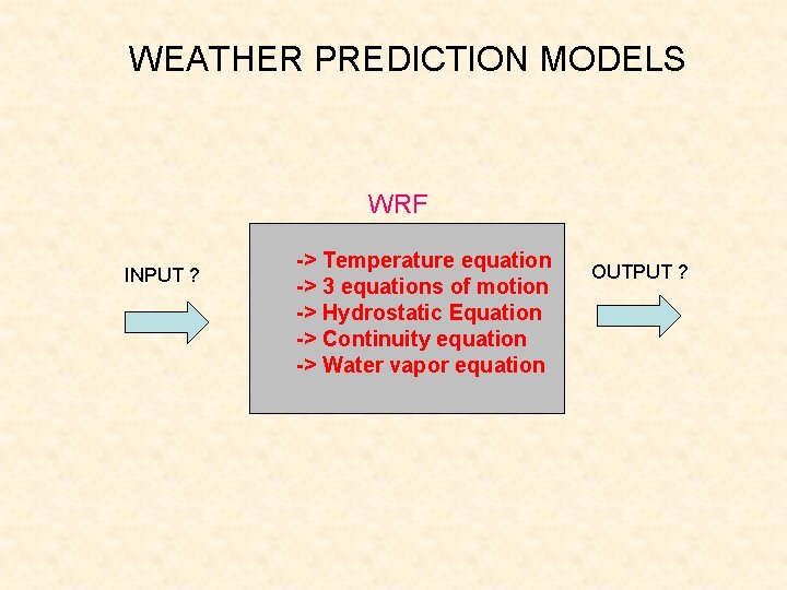
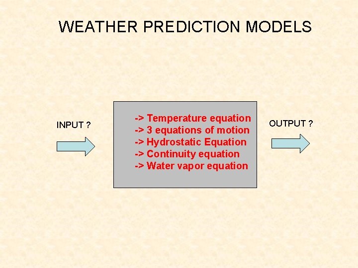
WEATHER PREDICTION MODELS WRF INPUT ? -> Temperature equation -> 3 equations of motion -> Hydrostatic Equation -> Continuity equation -> Water vapor equation OUTPUT ?

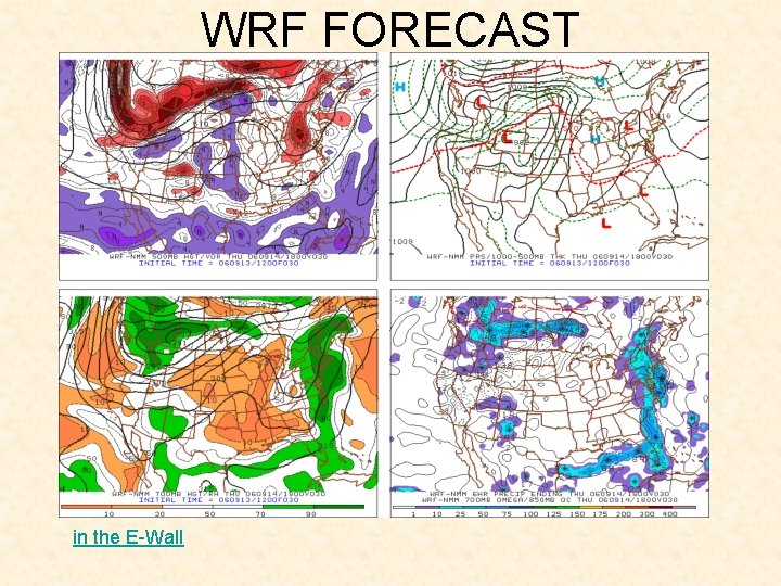
WRF FORECAST in the E-Wall

WEATHER PREDICTION MODELS INPUT ? -> Temperature equation -> 3 equations of motion -> Hydrostatic Equation -> Continuity equation -> Water vapor equation OUTPUT ?

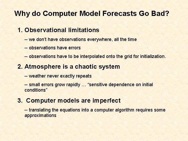
Why do Computer Model Forecasts Go Bad? 1. Observational limitations -- we don’t have observations everywhere, all the time -- observations have errors -- observations have to be interpolated onto the grid for initialization. 2. Atmosphere is a chaotic system -- weather never exactly repeats -- small errors grow rapidly … “sensitive dependence on initial conditions” 3. Computer models are imperfect -- translating the equations into a computer algorithm requires some approximations