ECE 753 FAULTTOLERANT COMPUTING Kewal K Saluja Department

ECE 753: FAULT-TOLERANT COMPUTING Kewal K. Saluja Department of Electrical and Computer Engineering Reliability Modeling and Analysis Lectures 8 -10 ECE 753 Fault Tolerant Computing

Overview • Recap • Introduction • Reliability Modeling – reliability block diagram – combinatorial model – Markov model • Other Parameters and analysis • General remarks and Summary ECE 753 Fault Tolerant Computing 2

Recap • Course introduction • Fundamental principles - Four types of redundancy • FEF and breaking FEF chain • Fault modeling – models at different levels, error models, process failure models • Testing and Test Generation – test generation, fault simulation, DFT and BIST concepts • Simple concepts in fault-tolerance – hardware redundancy, information redundancy, time redundancy, and software redundancy methods ECE 753 Fault Tolerant Computing 3

Introduction • References • [prad: 96] • [john: 89] • [triv: 82] These three books contain sufficient material covering this part of the course • Recap of definitions • Importance of analysis and analytical model • Mathematical formulation for quantitative analysis ECE 753 Fault Tolerant Computing 4

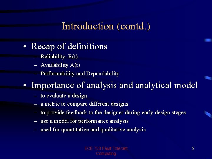
Introduction (contd. ) • Recap of definitions – Reliability R(t) – Availability A(t) – Performability and Dependability • Importance of analysis and analytical model – – – to evaluate a design a metric to compare different designs to provide feedback to the designer during early design stages use a model for performance analysis used for quantitative and qualitative analysis ECE 753 Fault Tolerant Computing 5

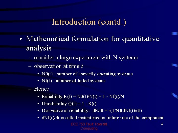
Introduction (contd. ) • Mathematical formulation for quantitative analysis – consider a large experiment with N systems – observation at time t • N 0(t) - number of correctly operating systems • Nf(t) - number of failed systems – Hence • • Reliability R(t) = N 0(t)/N(t) = 1 - Nf(t)/N Unreliability Q(t) = 1 - R(t) Derivative of reliability: d. R/dt = -(1/N)(d. Nf(t)/dt) d. Nf(t)/dt is called instantaneous failure rate of the component ECE 753 Fault Tolerant Computing 6

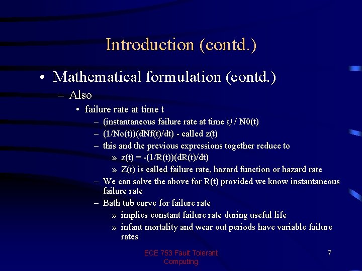
Introduction (contd. ) • Mathematical formulation (contd. ) – Also • failure rate at time t – (instantaneous failure rate at time t) / N 0(t) – (1/No(t))(d. Nf(t)/dt) - called z(t) – this and the previous expressions together reduce to » z(t) = -(1/R(t))(d. R(t)/dt) » Z(t) is called failure rate, hazard function or hazard rate – We can solve the above for R(t) provided we know instantaneous failure rate – Bath tub curve for failure rate » implies constant failure rate during useful life » infant mortality and wear out periods have variable failure rates ECE 753 Fault Tolerant Computing 7

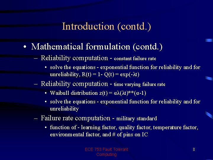
Introduction (contd. ) • Mathematical formulation (contd. ) – Reliability computation - constant failure rate • solve the equations - exponential function for reliability and for unreliability, R(t) = 1 - Q(t) = exp(-λt) – Reliability computation - time varying failure rate • Waibull distribution z(t) = αλ(λt)**(α-1) • solve the equations - exponential function for reliability and for unreliability – Failure rate computation - military standard • function of - learning factor, quality factor, temperature factor, environmental factor, and # of pins on IC ECE 753 Fault Tolerant Computing 8

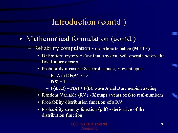
Introduction (contd. ) • Mathematical formulation (contd. ) – Reliability computation - mean time to failure (MTTF) • Definition: expected time that a system will operate before the first failure occurs • Probability measure: S-sample space, E-event space – for A in E P(A) >= 0 – P(S) = 1 – P(A B) = P(A) + P(B), when A and B are non-intersecting • Random Variable (RV) - X maps events of S to real-numbers • Probability distribution function of a RV • Probability density function (pdf) - derivative of the distribution function ECE 753 Fault Tolerant Computing 9

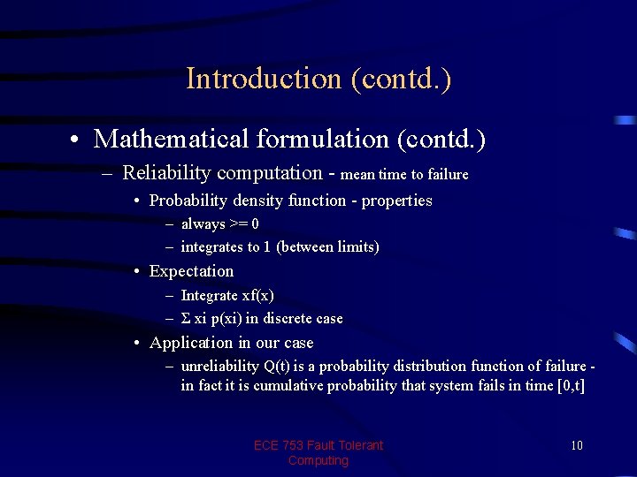
Introduction (contd. ) • Mathematical formulation (contd. ) – Reliability computation - mean time to failure • Probability density function - properties – always >= 0 – integrates to 1 (between limits) • Expectation – Integrate xf(x) – Σ xi p(xi) in discrete case • Application in our case – unreliability Q(t) is a probability distribution function of failure in fact it is cumulative probability that system fails in time [0, t] ECE 753 Fault Tolerant Computing 10

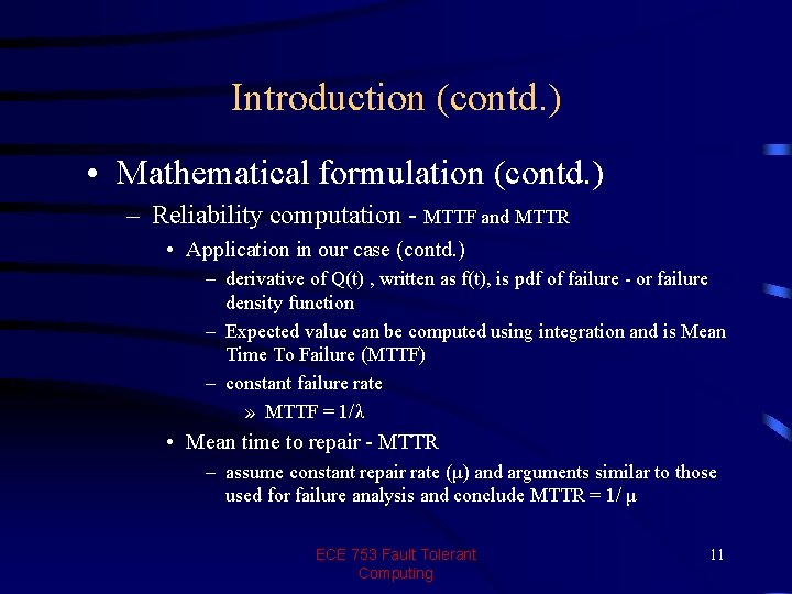
Introduction (contd. ) • Mathematical formulation (contd. ) – Reliability computation - MTTF and MTTR • Application in our case (contd. ) – derivative of Q(t) , written as f(t), is pdf of failure - or failure density function – Expected value can be computed using integration and is Mean Time To Failure (MTTF) – constant failure rate » MTTF = 1/λ • Mean time to repair - MTTR – assume constant repair rate (μ) and arguments similar to those used for failure analysis and conclude MTTR = 1/ μ ECE 753 Fault Tolerant Computing 11

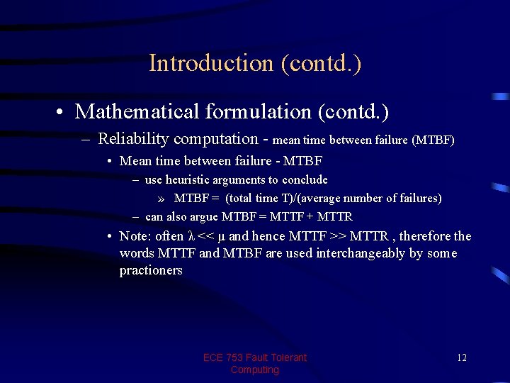
Introduction (contd. ) • Mathematical formulation (contd. ) – Reliability computation - mean time between failure (MTBF) • Mean time between failure - MTBF – use heuristic arguments to conclude » MTBF = (total time T)/(average number of failures) – can also argue MTBF = MTTF + MTTR • Note: often λ << μ and hence MTTF >> MTTR , therefore the words MTTF and MTBF are used interchangeably by some practioners ECE 753 Fault Tolerant Computing 12

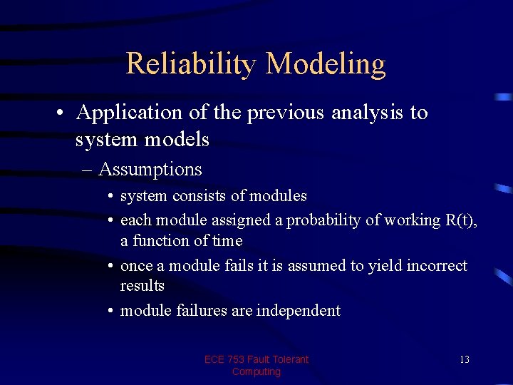
Reliability Modeling • Application of the previous analysis to system models – Assumptions • system consists of modules • each module assigned a probability of working R(t), a function of time • once a module fails it is assumed to yield incorrect results • module failures are independent ECE 753 Fault Tolerant Computing 13

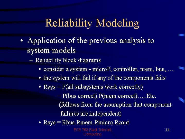
Reliability Modeling • Application of the previous analysis to system models – Reliability block diagrams • consider a system - micro. P, controller, mem, bus, … • the system will fail if any of the components fails • Rsys = P(all subsystems work correctly) = P(bus correct). P(mem correct)…. Etc. (follows from the assumption that component failures are independent) • Rsys = Rbus. Rmem. Rmicro. Rcont ECE 753 Fault Tolerant Computing 14

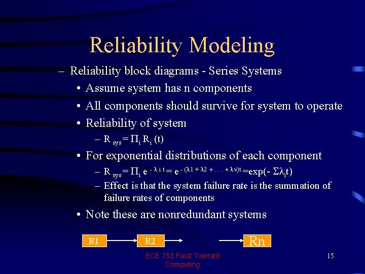
Reliability Modeling – Reliability block diagrams - Series Systems • Assume system has n components • All components should survive for system to operate • Reliability of system – R sys = Pi Ri (t) • For exponential distributions of each component – R sys = Pi e - l i t = e - (l 1 + l 2 +. . . + ln)t =exp(- Slit) – Effect is that the system failure rate is the summation of failure rates of components • Note these are nonredundant systems R 1 R 2 ECE 753 Fault Tolerant Computing Rn 15

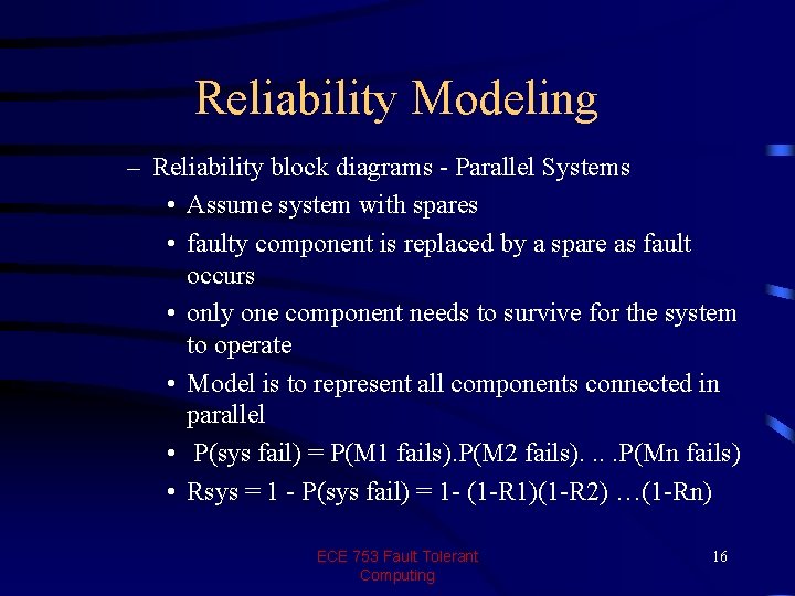
Reliability Modeling – Reliability block diagrams - Parallel Systems • Assume system with spares • faulty component is replaced by a spare as fault occurs • only one component needs to survive for the system to operate • Model is to represent all components connected in parallel • P(sys fail) = P(M 1 fails). P(M 2 fails). . P(Mn fails) • Rsys = 1 - P(sys fail) = 1 - (1 -R 1)(1 -R 2) …(1 -Rn) ECE 753 Fault Tolerant Computing 16

Reliability Modeling – Reliability block diagrams - Series-Parallel Systems • straight forward – Reliability block diagrams - MTTF of system • 1/(system failure rate) • Series systems - 1/(sum of individual falure rates) • Parallel systems and series parallel systems – work out by integration from the reliability or unreliability equations ECE 753 Fault Tolerant Computing 17

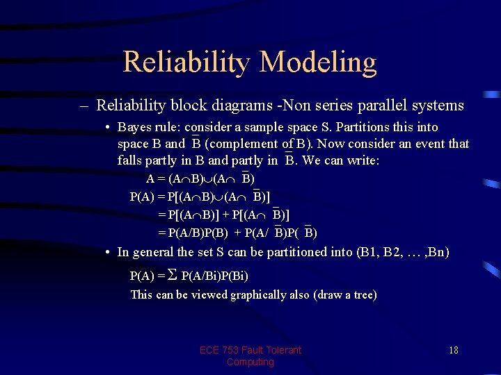
Reliability Modeling – Reliability block diagrams -Non series parallel systems • Bayes rule: consider a sample space S. Partitions this into space B and B (complement of B). Now consider an event that falls partly in B and partly in B. We can write: A = (A B) P(A) = P[(A B)] = P[(A B)] + P[(A B)] = P(A/B)P(B) + P(A/ B)P( B) • In general the set S can be partitioned into (B 1, B 2, … , Bn) P(A) = Σ P(A/Bi)P(Bi) This can be viewed graphically also (draw a tree) ECE 753 Fault Tolerant Computing 18

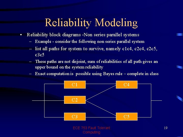
Reliability Modeling • Reliability block diagrams -Non series parallel systems – Example - consider the following non series parallel system – list all paths for system to survive, namely c 1 c 4, c 2 c 5, c 3 c 5 – These paths are not disjoint, sum of reliabilities of all path gives an upper bound on the system reliability – Exact computation is possible using Bayes rule – complete in class C 1 C 4 C 2 C 3 ECE 753 Fault Tolerant Computing C 5 19

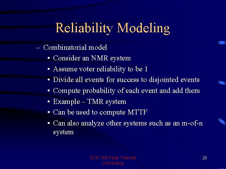
Reliability Modeling – Combinatorial model • Consider an NMR system • Assume voter reliability to be 1 • Divide all events for success to disjointed events • Compute probability of each event and add them • Example – TMR system • Can be used to compute MTTF • Can also analyze other systems such as an m-of-n system ECE 753 Fault Tolerant Computing 20

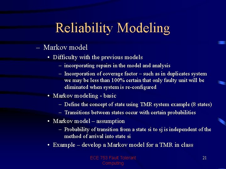
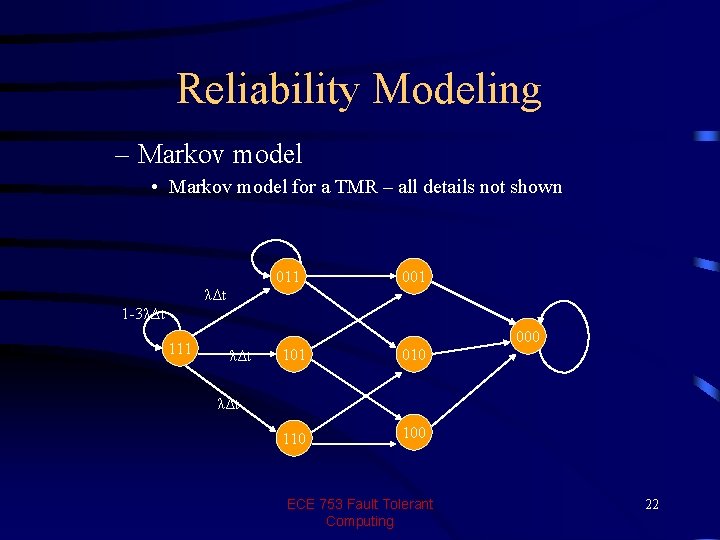
Reliability Modeling – Markov model • Difficulty with the previous models – incorporating repairs in the model and analysis – Incorporation of coverage factor – such as in duplicates system we may be less than 100% certain that only faulty unit will be eliminated when system is re-configured • Markov modeling - basic – Define the concept of state using TMR system example (8 states) – Transitions between states occur with certain probabilities • Markov model – assumption – Probability of transition from a state si to sj is independent of the method of arrival into state si • Example – develop a Markov model for a TMR in class ECE 753 Fault Tolerant Computing 21

Reliability Modeling – Markov model • Markov model for a TMR – all details not shown 011 001 λΔt 1 -3λΔt 111 000 λΔt 101 010 100 λΔt ECE 753 Fault Tolerant Computing 22

Reliability Modeling – Markov model- Reduced • Reduced Markov model for a TMR system • Previous eight state model can be reduced to a three state model by merging states and re-computing the transition probabilities – Markov model- accounting for repairs • We can include links between states knowing the repair rates of components ECE 753 Fault Tolerant Computing 23

Reliability Modeling – Markov model- analyzing systems • Consider a duplicate compare system – no repairs • Develop Markov model with 3 states • Develop a difference equation for computing probabilities for being in different states of the system • Develop a differential equation model • Solution methods – Numerical approach – Solving differential equation » direct approach » Using Laplace transforms ECE 753 Fault Tolerant Computing 24

Reliability Modeling – Markov model- analyzing systems • • Consider a duplicate compare system – with Develop Markov model with 3 states Develop a differential equation model Solve using Laplace transforms repairs – Yet one more example • duplicate compare system – with imperfect coverage • Develop Markov model with 5 states • Reduce model for different scenarios ECE 753 Fault Tolerant Computing 25

Other Parameters and analysis – Markov model- Can use other parameters • Safety – • Availability – Consider a simplex system – Develop Markov model with 2 states – Solve the system for probability of system being in available state – Define and compute steady state availability – Provide a intuitive explanation of the computed value of steady state availability and its relation of MTTF and MTTR • Maintainability ECE 753 Fault Tolerant Computing 26

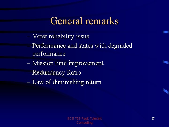
General remarks – Voter reliability issue – Performance and states with degraded performance – Mission time improvement – Redundancy Ratio – Law of diminishing return ECE 753 Fault Tolerant Computing 27

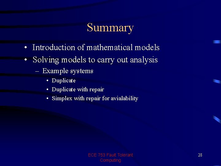
Summary • Introduction of mathematical models • Solving models to carry out analysis – Example systems • Duplicate with repair • Simplex with repair for avialability ECE 753 Fault Tolerant Computing 28