ECE 453 CS 447 SE 465 Software Testing

ECE 453 – CS 447 – SE 465 Software Testing & Quality Assurance Instructor Kostas Kontogiannis 1

Overview èStructural Testing èIntroduction – General Concepts èFlow Graph Testing èData Flow Testing èDefinitions èSome Basic Data Flow Analysis Algorithms èDefine/use Testing èSlice Based Testing èGuidelines and Observations èHybrid Methods èRetrospective on Structural Testing 2

Data Flow Testing • Data flow testing refers to a category of structural testing techniques that focus on the points of the code variables obtain values (are defined) and the points of the program these variables are referenced (are used) • We will focus on testing techniques that are centered – around faults that may occur when a variable is defined and referenced in not a proper way • A variable is defined but never used • A variable is used but never defined • A variable that is defined twice (or more times) before it is used – Parts of a program that constitute a slice – a subset of program statements that comply with a specific slicing criterion (i. e. all program statements that are affected by variable x at point P). 3

Fundamental Principles of Data Flow Analysis • Data flow analysis has been used extensively for compiler optimization algorithms • Data flow analysis algorithms are based on the analysis of variable usage in the basic blocks of the program’s Control Flow Graph (CFG) • We will focus in the next few slides on some basic data flow analysis terminology, and some basic data flow analysis algorithms • For the data flow analysis algorithms presented below the source of information is the book “Compilers – Principles, Techniques and Tools” by Aho, Sethi, and Ulman [1] 4

gen, kill, in, out Sets • Data flow analysis problems deal with the computation of specific properties of information related to definitions and uses of variables in basic blocks in the CFG. • There are different data flow analysis problems, and each one requires different information to be considered. • In general, we say that: – gen[B]: pertains to the information relevant to the problem and that is created in the block B – kill[B]: pertains to the information relevant to the problem and that is invalidated in the block B – in[B]: pertains to the information relevant to the problem and that holds upon entering the block B – out[B]: pertains to the information relevant to the problem and that holds upon exiting the block B 5

Reaching Definitions (1) • A definition of a variable x is a statement that assigns, or may assign, a value to x. The most common form of a definition is an assignment statement, or a read statement. These statements certainly define a value for the variable x and we refer to them as unambiguous definitions of the variable x • Unambiguous definitions have a strong impact on the problem of reaching definitions • There ambiguous definitions of a variable usually through: – Procedure call where x is passed by value is used as a global in the procedure – An assignment through a pointer (i. e. *p = y, if p points to x then we have an assignment to variable x) • So, what is the problem of reaching definitions? 6

Reaching Definitions (2) • We say that a definition d reaches a point p if there is a path following d to p, such that d is not killed, along that path • Intuitively, if a definition d of some variable x, reaches point p, then d might be the place at which the value of x used at p might have been defined • We kill a definition of a variable x if between two points along the path there is an unambiguous re-definition of x • For these types of problems we take conservative or “safe” solutions (i. e. all edges of the graph can be traversed – while in practice only one path will be traversed for a given execution) • In applications of reaching definitions it is normally conservative to assume that a definition can reach a point even if it might not. Thus, we allow paths that may never be traversed in any execution of a program, and we allow definitions to pass through ambiguous definitions of the same variable [1] 7

gen, kill, in, out for Reaching Definitions • gen[S], where S is a basic block (node) in the program’s Control Flow Graph, is the set of definitions generated by S. That is a definition d (e. g. a=b+c) in S reaches the end of S via a path that does not go outside S. • kill[S], is the set of definitions that never reach the end of S, event if they reach the beginning. In order for a definition d to be in the set kill[S], – every path from the beginning to end of S must have an unambiguous definition of the same variable defined by d (note d may be “input” to S by another basic block), and – if d appears in S (i. e. the definition is a statement in the basic block S), then following every occurrence of d along any path must be another definition in S of the same variable. 8

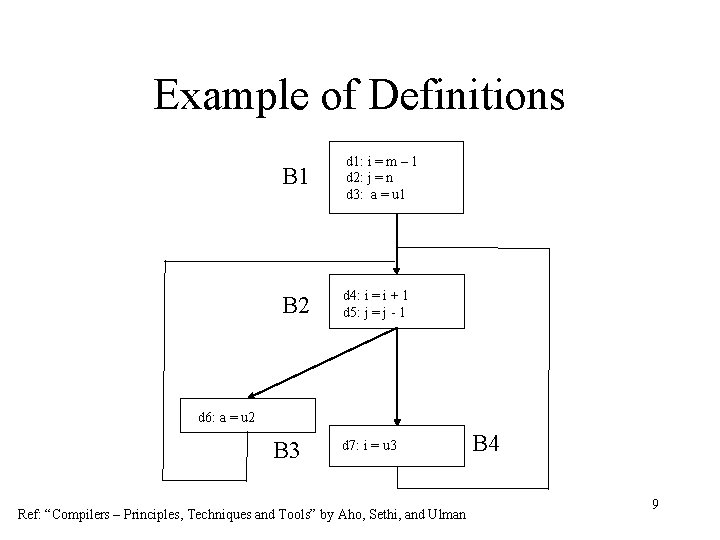
Example of Definitions B 1 d 1: i = m – 1 d 2: j = n d 3: a = u 1 B 2 d 4: i = i + 1 d 5: j = j - 1 d 6: a = u 2 B 3 d 7: i = u 3 Ref: “Compilers – Principles, Techniques and Tools” by Aho, Sethi, and Ulman B 4 9

gen and kill Principles in Data Flow Analysis (1) s d 1: a=b+c gen[S] = {d 1} kill[S] = Da – {d} out[S] = gen[S] U (in[S] – kill[S]) s 1 s = s 2 gen[S] = gen[S 2] U (gen[S 1] – kill[S 2]) kill[S] = kill[S 2] U (kill[S 1] – gen[S 2]) in[S 1] = in[S] in[S 2] = out[S 1] out[S] = out[S 2] 10

Gen and Kill Principles in Data Flow Analysis (2) gen[S] = gen[S 1] U gen[S 2] kill[S] = kill[S 1] ∩ kill[S 2] s = s 1 s 2 in[S 1] = in[S 2] = in[S] out[S] = out[S 1] U out[S 2] gen[S] = gen[S 1] kill[S] = kill[S 1] s = s 1 in[S 1] = in[S] U out[S 1] out[S] = out[S 1] where, 11 out[S 1] = gen[S 1] U (in[S 1] – kill[S 1])

Conservative Estimation of Data Flow Information • In data flow analysis we assume that the statements are “un-interpreted” (i. e. both then and the else parts of an if-statement are considered in the analysis while in practice during execution only one branch is taken) • For each data flow analysis problem we must examine the effect of inaccurate estimates • We generally accept discrepancies that are safe in the sense that they may not provide inaccurate information in the context of applying an optimization, devising a test case, or revealing dependencies between program statements • In the previous example (reaching definitions) the “true” gen is a subset of the computed gen, and the “true” kill is a superset of the computed kill. Intuitively, increasing gen, adds to the set of definitions that can reach a point, and cannot prevent a definition from reaching a place if it can be truly reached. The same holds for decreasing the kill set. 12

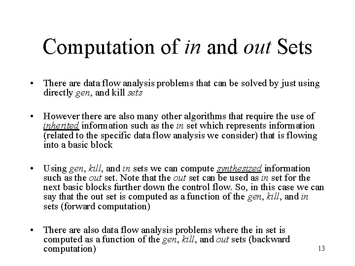
Computation of in and out Sets • There are data flow analysis problems that can be solved by just using directly gen, and kill sets • However there also many other algorithms that require the use of inherited information such as the in set which represents information (related to the specific data flow analysis we consider) that is flowing into a basic block • Using gen, kill, and in sets we can compute synthesized information such as the out set. Note that the out set can be used as in set for the next basic blocks further down the control flow. So, in this case we can say that the out set is computed as a function of the gen, kill, and in sets (forward computation) • There also data flow analysis problems where the in set is computed as a function of the gen, kill, and out sets (backward computation) 13

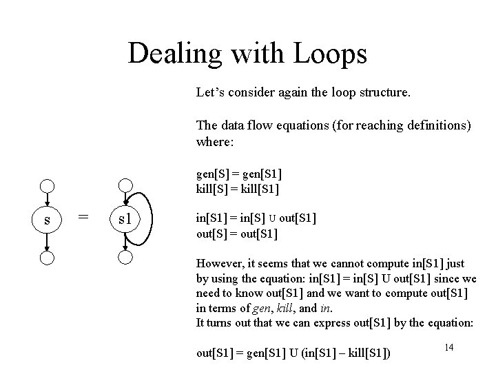
Dealing with Loops Let’s consider again the loop structure. The data flow equations (for reaching definitions) where: gen[S] = gen[S 1] kill[S] = kill[S 1] s = s 1 in[S 1] = in[S] U out[S 1] out[S] = out[S 1] However, it seems that we cannot compute in[S 1] just by using the equation: in[S 1] = in[S] U out[S 1] since we need to know out[S 1] and we want to compute out[S 1] in terms of gen, kill, and in. It turns out that we can express out[S 1] by the equation: out[S 1] = gen[S 1] U (in[S 1] – kill[S 1]) 14

Iterative Algorithm for Reaching Definitions (1) • Input: A flow graph for which kill[B] and gen[B] have been computed for each basic block B of the graph • Output: in[B] and out[B] sets for each basic block B • Method: An iterative algorithm, starting with an “estimate” in[B] = for all B and converging to the desired values of in and out sets. A Boolean variable records whether we have achieved a “stable” state that is in consecutive iterations we have no changes in the in and out sets, that is we have achieved convergence. Ref: “Compilers – Principles, Techniques and Tools” by Aho, Sethi, and Ulman 15

Iterative Algorithm for Reaching Definitions (2) for each block B do in[B] = O for each block B do out[B] = gen[B] change = true; while change do begin change = false; for each block B do begin in[B] = UP (where P is a predecessor of B) out[P] oldout – out[B]; out[B] = gen[B] U (in[B] – kill[B]); if out[B]≠ oldout then change = true end Ref: “Compilers – Principles, Techniques and Tools” by Aho, Sethi, and Ulman 16

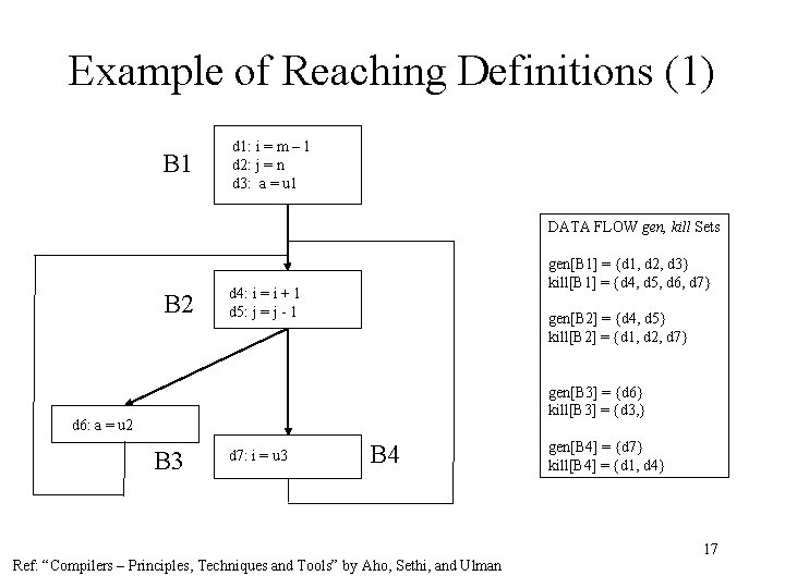
Example of Reaching Definitions (1) B 1 d 1: i = m – 1 d 2: j = n d 3: a = u 1 DATA FLOW gen, kill Sets B 2 gen[B 1] = {d 1, d 2, d 3} kill[B 1] = {d 4, d 5, d 6, d 7} d 4: i = i + 1 d 5: j = j - 1 gen[B 2] = {d 4, d 5} kill[B 2] = {d 1, d 2, d 7} gen[B 3] = {d 6} kill[B 3] = {d 3, } d 6: a = u 2 B 3 d 7: i = u 3 B 4 Ref: “Compilers – Principles, Techniques and Tools” by Aho, Sethi, and Ulman gen[B 4] = {d 7} kill[B 4] = {d 1, d 4} 17

Example of Reaching Definitions (2) Initial Pass 1 Pass 2 Block in[B] out[B] B 1 000 0000 111 0000 B 2 0000 000 111 001 1110 1111 001 1110 B 3 0000 0010 001 1110 000 1110 B 4 0000 0001 001 1110 001 0111 18

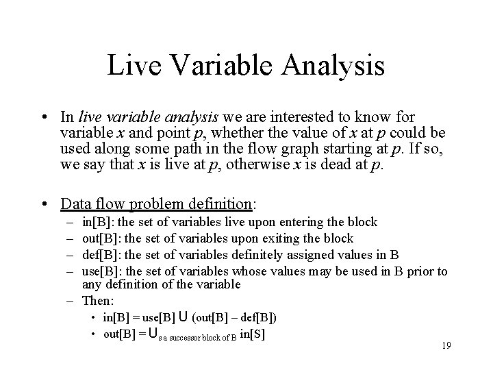
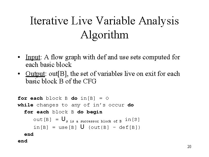
Live Variable Analysis • In live variable analysis we are interested to know for variable x and point p, whether the value of x at p could be used along some path in the flow graph starting at p. If so, we say that x is live at p, otherwise x is dead at p. • Data flow problem definition: – – in[B]: the set of variables live upon entering the block out[B]: the set of variables upon exiting the block def[B]: the set of variables definitely assigned values in B use[B]: the set of variables whose values may be used in B prior to any definition of the variable – Then: • in[B] = use[B] U (out[B] – def[B]) • out[B] = Us a successor block of B in[S] 19

Iterative Live Variable Analysis Algorithm • Input: A flow graph with def and use sets computed for each basic block • Output: out[B], the set of variables live on exit for each basic block B of the CFG for each block B do in[B] = O while changes to any of in’s occur do for each block B do begin out[B] = Us is a successor block of B in[S] in[B] = use[B] U (out{B] – def[B]) end 20

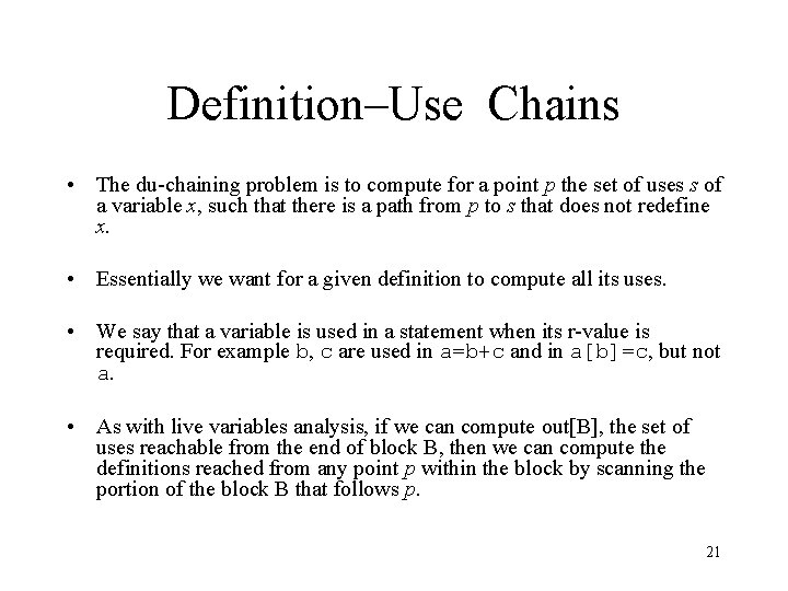
Definition–Use Chains • The du-chaining problem is to compute for a point p the set of uses s of a variable x, such that there is a path from p to s that does not redefine x. • Essentially we want for a given definition to compute all its uses. • We say that a variable is used in a statement when its r-value is required. For example b, c are used in a=b+c and in a[b]=c, but not a. • As with live variables analysis, if we can compute out[B], the set of uses reachable from the end of block B, then we can compute the definitions reached from any point p within the block by scanning the portion of the block B that follows p. 21

Def-use Chains • Data flow problem definition: – in[B]: the set of definitions reached from the beginning of block B – out[B]: out[B], the set of uses reachable from the end of block B – def[B]: The set of pairs <s, x> such that s is a statement which uses x, s is nit in B, and B has a definition of x. – upward_use[B]: the set of pairs <s, x> such that s is a statement in B which uses variable x and such that no prior definition of x occurs in B. – Then: • in[B] = upward_use[B] U (out[B] – def[B]) • out[B] = Us a successor block of B in[S] • The iterative algorithm is similar to the one used for live variables analysis 22

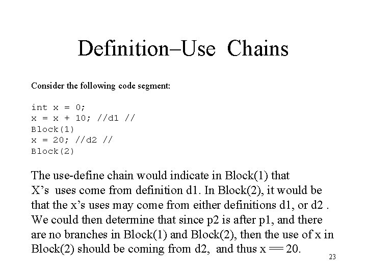
Definition–Use Chains Consider the following code segment: int x = 0; x = x + 10; //d 1 // Block(1) x = 20; //d 2 // Block(2) The use-define chain would indicate in Block(1) that X’s uses come from definition d 1. In Block(2), it would be that the x’s uses may come from either definitions d 1, or d 2. We could then determine that since p 2 is after p 1, and there are no branches in Block(1) and Block(2), then the use of x in Block(2) should be coming from d 2, and thus x == 20. 23