ECE 453 CS 447 SE 465 Software Testing

ECE 453 – CS 447 – SE 465 Software Testing & Quality Assurance Instructor Kostas Kontogiannis 1

Overview èSoftware Reverse Engineering èReliability and Availability èSoftware Reliability Models èCalendar Time, Execution Time èOperational Phase èConcurrent Components 2

S/W Reliability • Basic definitions: • S/W reliability: probability that the software will not cause a failure for some specified time. • Failure: divergence in expected external behavior. • Fault: a bug (incorrect intermediate state). • Error: a programmer mistake (misinterpretation of specifications? ) 3

S/W Reliability • Basic question: how to estimate the growth in s/w reliability as its errors are being removed. • Major issues: • testing - (how much? When to stop!) • field use ( # of trained personnel? Support staff? ) • S/W reliability growth models: observe past failure history and give an estimate of the future failure behavior. About 40 models have been proposed. 4

Reliability and Availability • A simple measure of reliability can be given as: MTBF = MTTF + MTTR , where MTBF is mean time between failures MTTF is mean time to fail MTTR is mean time to repair 5

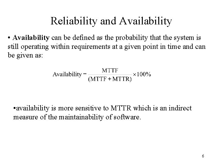
Reliability and Availability • Availability can be defined as the probability that the system is still operating within requirements at a given point in time and can be given as: • availability is more sensitive to MTTR which is an indirect measure of the maintainability of software. 6

Reliability and Availability • Since each error in the program does not have the same failure rate, – the total error count does not provide a good indication of the reliability of the system. • MTBF is perhaps more useful (meaningful) than defects/KLOC since the user is concerned with failures not the total error count. 7

Software Reliability Models • Software reliability models can be classified into many different groups; some of the more prominent (better known) groups include: • error seeding - estimates the number of errors in a program. Errors are divided into indigenous errors and induced (seeded) errors. The unknown number of indigenous errors is estimated from the number of induced errors and the ratio of the two types of errors obtained from the testing data. 8

Software Reliability Models • Reliability growth • Measures and predicts the improvement of reliability through the testing process using a growth function to represent the process. • Independent variables of the growth function could be time, number of test cases (or testing stages) and • The dependent variables can be reliability, failure rate or cumulative number of errors detected. 9

Software Reliability Models • Nonhomogeneous Poisson process (NHPP) – provide an analytical framework for describing the software failure phenomenon during testing. – the main issue is to estimate the mean value function of the cumulative number of failures experienced up to a certain point in time. – a key example of this approach is the series of Musa models 10

Software Reliability Models • A typical measure (failures per unit time) is the failure intensity (rate) given as: • where = program CPU time (in a time shared computer) or wall clock time (in an embedded system). 11

Software Reliability Models • SRG models are generally “black box” - no easy way to account for a change in the operational profile – consequences are that we are unable to go from test to field 12

Software Reliability Models · Many models have been proposed, perhaps the most prominent are: Musa Basic model Musa/Okomoto Logarithmic model • Some models work better than others depending on the application area and operating characteristics: i. e. interactive? data intensive? control intensive? real-time? 13

Basic Assumptions of Musa 1. Errors in the program are independent and distributed with constant average occurrence rate. 2. Execution time between failures is large with respect to instruction execution time. 3. Potential ‘test space’ covers it ‘use space’. 4. The set of inputs per test run (test or operational) is randomly selected. 5. All failures are observed. 6. The error causing the failure is immediately fixed or else its re -occurrence is not counted again. 14

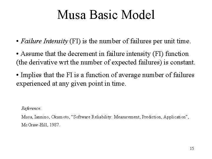
Musa Basic Model • Failure Intensity (FI) is the number of failures per unit time. • Assume that the decrement in failure intensity (FI) function (the derivative wrt the number of expected failures) is constant. • Implies that the FI is a function of average number of failures experienced at any given point in time. Reference: Musa, Iannino, Okumoto, “Software Reliability: Measurement, Prediction, Application”, Mc. Graw-Hill, 1987. 15

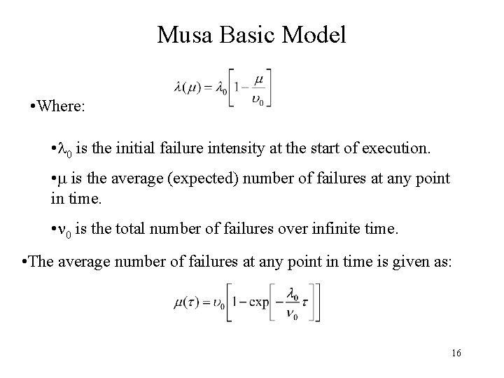
Musa Basic Model • Where: • 0 is the initial failure intensity at the start of execution. • is the average (expected) number of failures at any point in time. • 0 is the total number of failures over infinite time. • The average number of failures at any point in time is given as: 16

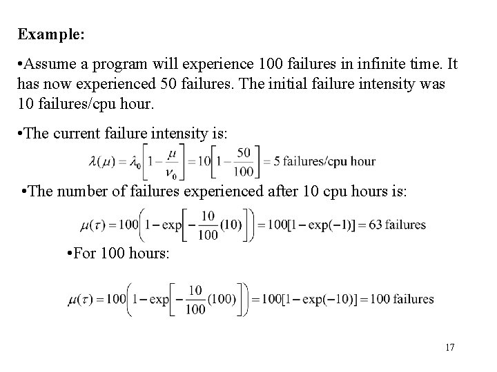
Example: • Assume a program will experience 100 failures in infinite time. It has now experienced 50 failures. The initial failure intensity was 10 failures/cpu hour. • The current failure intensity is: • The number of failures experienced after 10 cpu hours is: • For 100 hours: 17

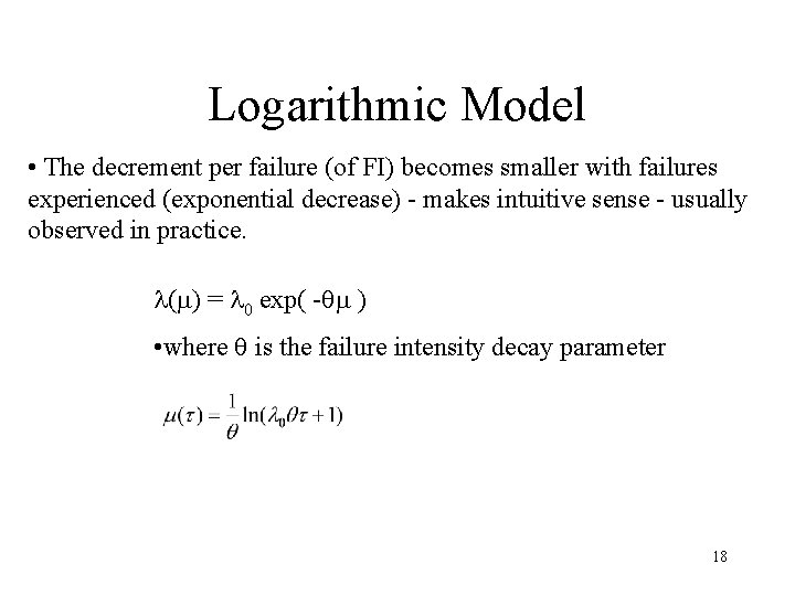
Logarithmic Model • The decrement per failure (of FI) becomes smaller with failures experienced (exponential decrease) - makes intuitive sense - usually observed in practice. ( ) = 0 exp( - ) • where is the failure intensity decay parameter 18

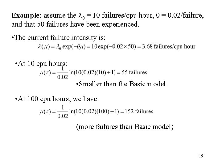
Example: assume the 0 = 10 failures/cpu hour, = 0. 02/failure, and that 50 failures have been experienced. • The current failure intensity is: • At 10 cpu hours: • Smaller than the Basic model • At 100 cpu hours, we have: (more failures than Basic model) 19

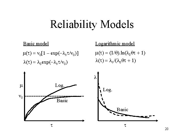
Reliability Models Basic model Logarithmic model ( ) = v 0[1 – exp(- 0 /v 0)] ( ) = (1/ ). ln( 0 + 1) ( ) = 0 exp(- 0 /v 0) ( ) = 0/( 0 + 1) Log. v 0 Log. Basic 20

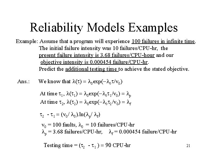
Reliability Models Example: Assume that a program will experience 100 failures in infinite time. The initial failure intensity was 10 failures/CPU-hr, the present failure intensity is 3. 68 failures/CPU-hour and our objective intensity is 0. 000454 failure/CPU-hr. Predict the additional testing time to achieve the stated objective. Ans. : We know that ( ) = 0 exp(- 0 /v 0) At time 1, ( 1) = 0 exp(- 0 1/v 0) = p At time 2, ( 2) = 0 exp(- 0 2/v 0) = f 2 - 1 = (v 0/ 0). ln( p/ f) v 0 = 100 faults, 0 = 10 failures/CPU-hr p = 3. 68 failures/CPU-hr, f = 0. 000454 failure/CPU-hr Testing time = ( 2 - 1 ) = 90 CPU-hr 21

Choice of Model Basic Model: • for studies or predictions before execution and failure data available • using study of faults to determine effects of a new s/w engineering technology • the program size is changing continually or substantially (i. e. during integration) 22

Logarithmic Model • system subjected to highly non-uniform operational profiles. • highly predictive validity is needed early in the execution period. The rapidly changing slope of the failure intensity during early stages can be better fitted with the logarithmic Poisson than the basic model. • basic idea: use the basic model for pretest studies and estimates and periods of evolution while switching to the logarithmic model when integration is complete. 23

Calendar Time Component • The calendar time component attempts to relate execution time and calendar time by determining at any given time the ratio: • The calendar time is obtaining by integrating this ratio with respect to execution time. • The calendar time is of most concern during the test and repair phases as well to predict the dates at which given failure intensities will be achieved 24

• The calendar time is based on a debugging process model and takes into account the following: • The resources used in running the program for a given execution time and processing a specified quantity of features; • The resource quantities available; • The degree to which a resource can be utilized (due to possible bottlenecks) during the period in which it is limiting. 25

• At the start of testing: a large number of failures in short time intervals; q Stop testing to allow fixing of faults. • As testing progresses, q the intervals between faults is longer, q failure correction people not filled with work q the test team becomes the bottleneck and q eventually the computing resources are the limiting factor. 26

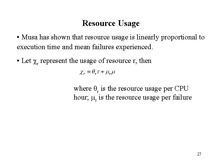
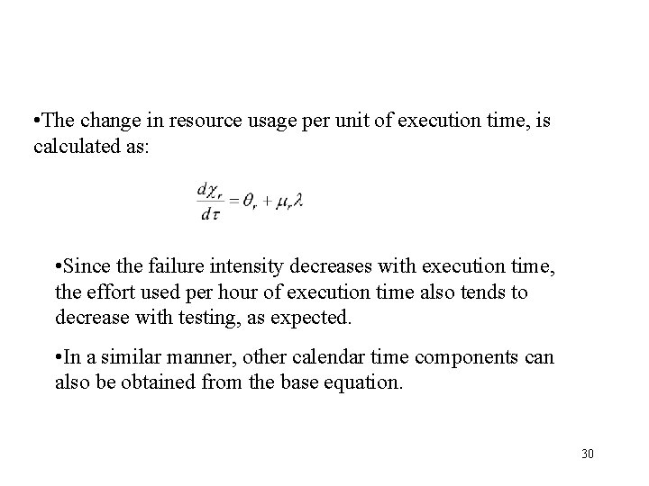
Resource Usage • Musa has shown that resource usage is linearly proportional to execution time and mean failures experienced. • Let r represent the usage of resource r, then where r is the resource usage per CPU hour; r is the resource usage per failure 27

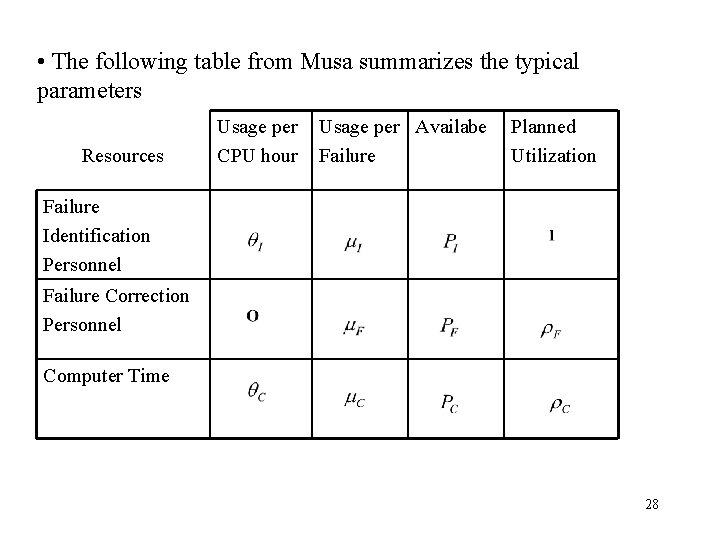
• The following table from Musa summarizes the typical parameters Resources Usage per CPU hour Usage per Availabe Failure Planned Utilization Failure Identification Personnel Failure Correction Personnel Computer Time 28

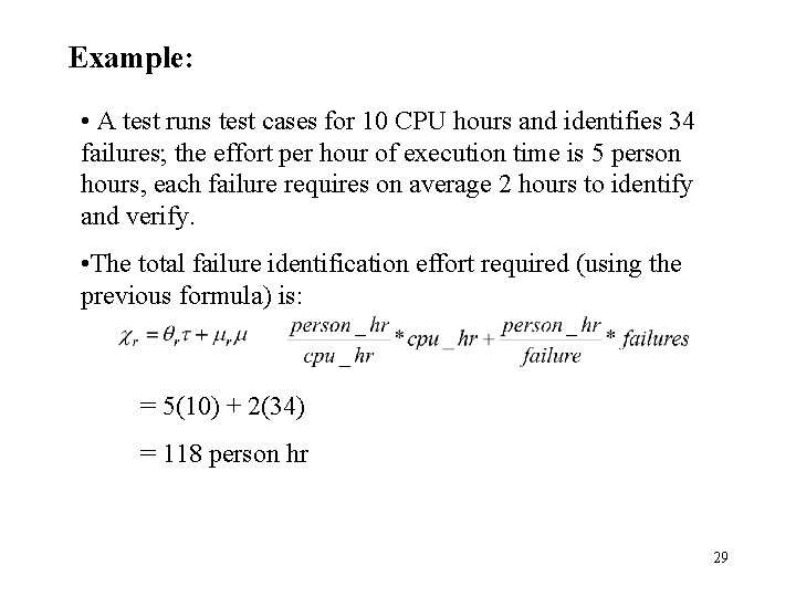
Example: • A test runs test cases for 10 CPU hours and identifies 34 failures; the effort per hour of execution time is 5 person hours, each failure requires on average 2 hours to identify and verify. • The total failure identification effort required (using the previous formula) is: = 5(10) + 2(34) = 118 person hr 29

• The change in resource usage per unit of execution time, is calculated as: • Since the failure intensity decreases with execution time, the effort used per hour of execution time also tends to decrease with testing, as expected. • In a similar manner, other calendar time components can also be obtained from the base equation. 30

Operational Phase • Once the software has been released and is operational, and no features are added or repairs made between releases, the failure intensity will become a constant. • Both models reduce to a homogeneous Poisson processes with the failure intensity as the parameter. The failures in a given time period follow a Poisson distribution while the failure intervals follow an exponential distribution. 31

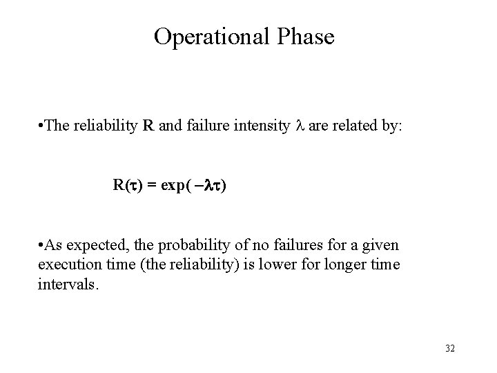
Operational Phase • The reliability R and failure intensity are related by: R( ) = exp( ) • As expected, the probability of no failures for a given execution time (the reliability) is lower for longer time intervals. 32

Operational Phase • In many cases, the operational phase consists of a series of releases – results in the reliability and failure intensity to be a series of step functions; – under these cases, if the releases are frequent and the failure intensity decreases, • step functions can be approximated by one the previous reliability models 33

Operational Phase • We can also apply the reliability models directly to reported failures (not counting repetitions) – but that now the model reflects the case when failures have been corrected • If failures corrected in the field, then the model is similar to that of the system test phase 34

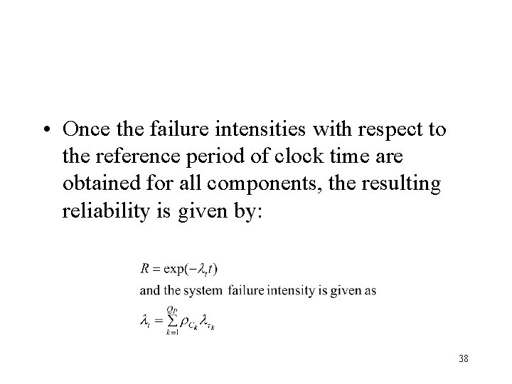
System Reliability (Concurrent Components) • Assume that we have QP components with constant failure intensities where their reliabilities are measured over a common calendar time interval and that all must function correctly for system success, then the system failure intensity is given by where k refers to the individual component failure intensities. 35

• Software reliabilities are usually given in terms of execution time • Before software and hardware reliabilities are combined, the conversion of software reliability is required. • First convert the reliability R of each software component to failure intensity. • Using to represent failure intensity as being with respect to execution time, we obtain using R( ) = exp( ) where is the execution time period for which the reliability was given. 36

§ Now let C be the average utilization by the program of the machine q assuming that it does not vary greatly over the failure intervals, qthen the failure intensity with respect to clock time t is given by: § Note that the average utilization is less than or equal to 1. 37

• Once the failure intensities with respect to the reference period of clock time are obtained for all components, the resulting reliability is given by: 38

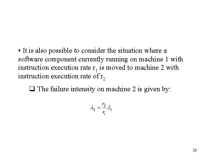
• It is also possible to consider the situation where a software component currently running on machine 1 with instruction execution rate r 1 is moved to machine 2 with instruction execution rate of r 2 q The failure intensity on machine 2 is given by: 39