Early estimates Manca Golmajer Statistical Office of the


 • Input 1: time series of interest (aggregate data) time TSI 2008")
 • Input 2: time series of enterprise data (microdata) time P 001")
 • Model: 2 stages: 1. Principal component analysis (PCA) - dimensionality reduction")
 • Output: – An estimate for the series of interest‘s last point")
 • Many possibilities for improving the models: – Length of time series")
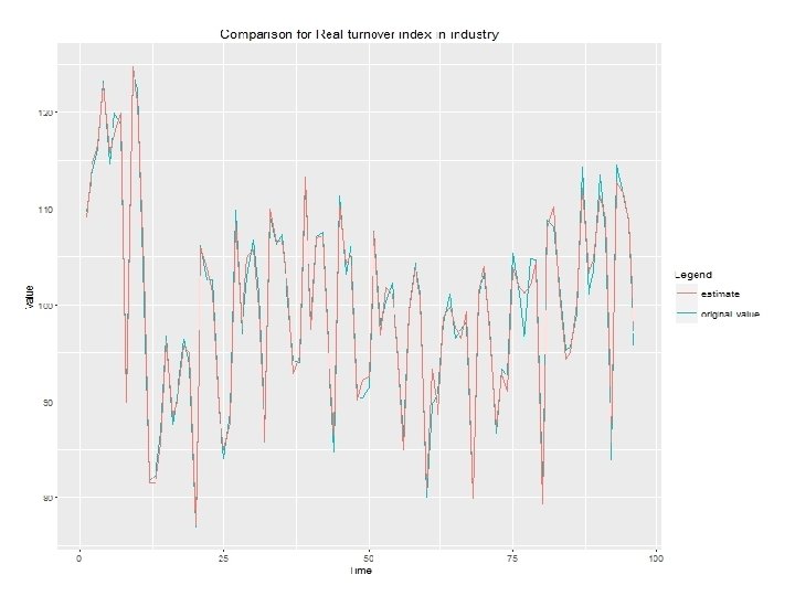
 Example 1: Estimation of the last period - Time")
 Example 2: Estimation of the last periods under various")
 - Conclusions: - C 1: - 14─56 principal components")
- Slides: 13
Early estimates Manca Golmajer Statistical Office of the Republic of Slovenia 13 October 2016
ESSnet on Big Data: WP 6: Early estimates Aim: • Investigate multiple data sources (big data, official statistical data, administrative data, etc. ). • Use combined data sources to create early estimates for statistics. • Describe the process for the most promising combinations.
Overview of possible sources to be investigated Big Data Registers and existing sources Surveys Job vacancies adds from job portals Statistical Register of Employment Turnover data from various short-term surveys Traffic loops Data from the Employment Agency Consumer confidence index Social media data (Twitter, Facebook, etc. ) Tax data Business tendency Supermarket scanner data Wages and salaries … News feeds/messages … …
Nowcasting turnover indices • One of the pilots that was started in WP 6. • Statistics Finland (Henri Luomaranta et al. ) • Interesting methodological suggestions for estimating early economic indicators → SURS decided for testing starting with this idea. • Modelling isn‘t new, but it is very often used in connection with big data sources. • Modelling is very useful for estimating early economic indicators based on many different data sources.
Model (1) • Input 1: time series of interest (aggregate data) time TSI 2008 M 01 109. 64 2008 M 02 113. 51 2008 M 03 116. 23 … 2015 M 12 … 95. 78
Model (2) • Input 2: time series of enterprise data (microdata) time P 001 P 002 … P 973 2008 M 01 3526 214 … 66519 2008 M 02 4252 332 … 36012 2008 M 03 4111 411 … 52447 … … 5241 412 … 71025 … 2015 M 12
Model (3) • Model: 2 stages: 1. Principal component analysis (PCA) - dimensionality reduction - time series of enterprise data → standardize → choose the first few principal components 2. Linear regression - Y (dependent variable): time series of interest, e. g. turnover index - X 1, …, Xn (predictors): e. g. the chosen principal components
Model (4) • Output: – An estimate for the series of interest‘s last point in time: e. g. 2015 M 12 – Others, e. g. : • Percentage of variability of the data explained by the chosen principal components • Percentage of variability of the time series of interest explained by the chosen linear regression model • Mean absolute error of the chosen linear regression model
Model (5) • Many possibilities for improving the models: – Length of time series – Data editing (e. g. imputations) – Choice of principal components – Additional predictors in linear regression • Many issues: – Availability of the data – Software: RStudio – Quality of the model
First results of testing (1) Example 1: Estimation of the last period - Time series of interest: Real turnover index in industry - Time series of enterprise data: Real turnover of 973 industrial enterprises - Data: from 2008 M 01 to 2015 M 12 (8 years) - Principal component analysis: - 33 chosen principal components explain 80. 2% of the variability of enterprise data - Linear regression: - 97. 5% of variability of real turnover index in industry is explained Maximum absolute error: 4. 94 Mean absolute error: 1. 04 Standard deviation of error: 1. 32 The last period is 2015 M 12: Original value: 95. 78 Estimate: 97. 18 Absolute error: 1. 40
First results of testing (2) Example 2: Estimation of the last periods under various conditions - Time series of interest: Real turnover index in industry - Time series of enterprise data: Real turnover of industrial enterprises - Data: from 2008 M 01 to 2013 M 01─2015 M 12 (5─8 years) - Principal component analysis: - Various conditions for choosing principal components: - C 1: The chosen principal components explain at least 70% (75%, 80%, 85%, 90%) of variability of enterprise data. - C 2: Time series in the linear regression model are at least 7 (8, 10, 15, 20) times longer than the number of the chosen principal components. - C 3: The last chosen principal component explains at least 5% of variability of enterprise data.
First results of testing (3) - Conclusions: - C 1: - 14─56 principal components are chosen. - More than 96% of variability of real turnover index in industry is explained. - The last period: Mean absolute relative error: 1. 8%─2. 7% Maximum absolute relative error: 5. 2%─10. 4% The errors are often greater than expected. - C 2: - 3─13 principal components are chosen. - More than 88% of variability of real turnover index in industry is explained. - The last period: Mean absolute relative error: 2. 1%─2. 7% Maximum absolute relative error: 5. 5%─8. 3% The errors are often greater than expected. - C 3: not very promising - „ 70%“, „ 75%“, „ 7 times“, „ 8 times“ seem to be the most promising.