Digital Image Processing Lecture 9 Filtering in Frequency

Digital Image Processing Lecture 9: Filtering in Frequency Domain Prof. Charlene Tsai

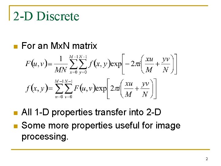
2 -D Discrete n For an Mx. N matrix n All 1 -D properties transfer into 2 -D Some more properties useful for image processing. n 2

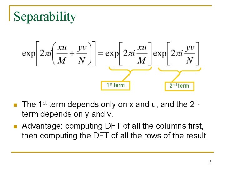
Separability 1 st term n n 2 nd term The 1 st term depends only on x and u, and the 2 nd term depends on y and v. Advantage: computing DFT of all the columns first, then computing the DFT of all the rows of the result. 3

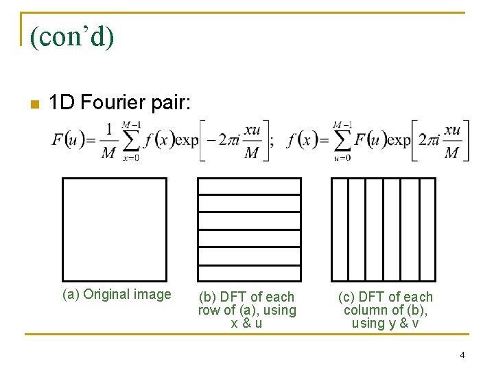
(con’d) n 1 D Fourier pair: (a) Original image (b) DFT of each row of (a), using x&u (c) DFT of each column of (b), using y & v 4

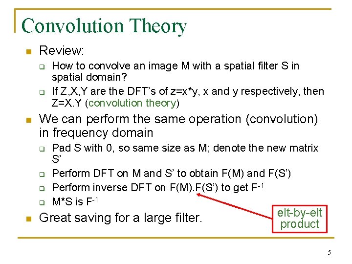
Convolution Theory n Review: q q n We can perform the same operation (convolution) in frequency domain q q n How to convolve an image M with a spatial filter S in spatial domain? If Z, X, Y are the DFT’s of z=x*y, x and y respectively, then Z=X. Y (convolution theory) Pad S with 0, so same size as M; denote the new matrix S’ Perform DFT on M and S’ to obtain F(M) and F(S’) Perform inverse DFT on F(M). F(S’) to get F-1 M*S is F-1 Great saving for a large filter. elt-by-elt product 5

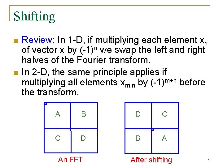
Shifting n n Review: In 1 -D, if multiplying each element xn of vector x by (-1)n we swap the left and right halves of the Fourier transform. In 2 -D, the same principle applies if multiplying all elements xm, n by (-1)m+n before the transform. A B D C C D B A An FFT After shifting 6

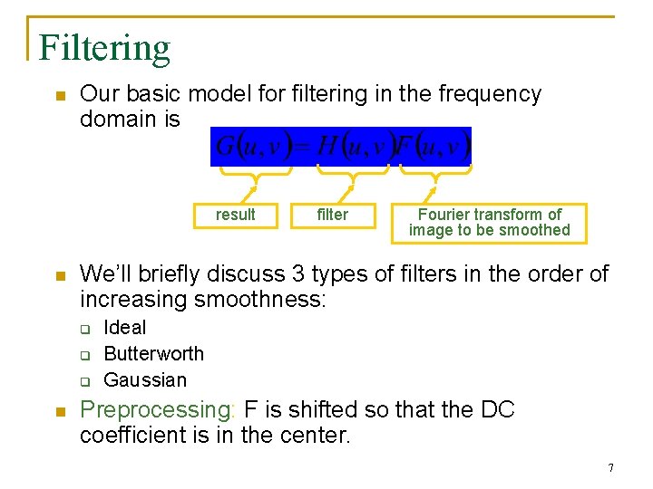
Filtering n Our basic model for filtering in the frequency domain is result n Fourier transform of image to be smoothed We’ll briefly discuss 3 types of filters in the order of increasing smoothness: q q q n filter Ideal Butterworth Gaussian Preprocessing: F is shifted so that the DC coefficient is in the center. 7

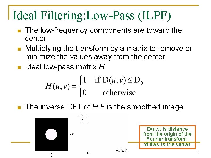
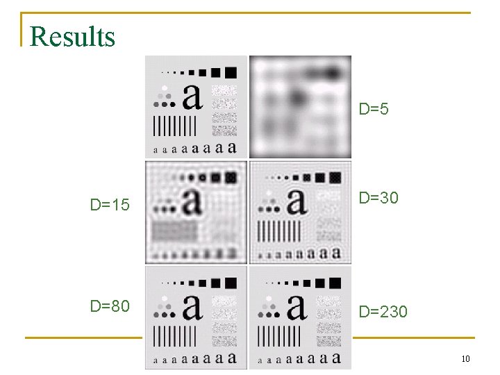
Ideal Filtering: Low-Pass (ILPF) n The low-frequency components are toward the center. Multiplying the transform by a matrix to remove or minimize the values away from the center. Ideal low-pass matrix H n The inverse DFT of H. F is the smoothed image. n n D(u, v) is distance from the origin of the Fourier transform, shifted to the center 8

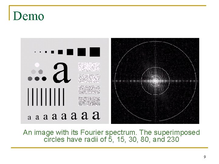
Demo An image with its Fourier spectrum. The superimposed circles have radii of 5, 15, 30, 80, and 230 9

Results D=5 D=15 D=30 D=80 D=230 10

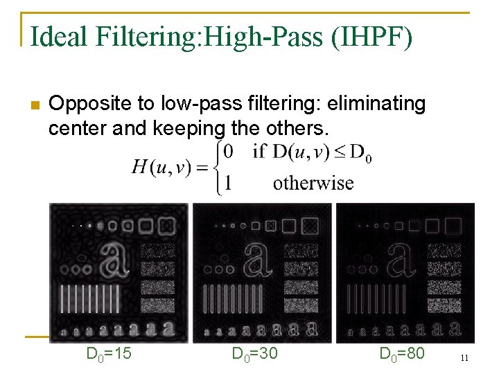
Ideal Filtering: High-Pass (IHPF) n Opposite to low-pass filtering: eliminating center and keeping the others. D 0=15 D 0=30 D 0=80 11

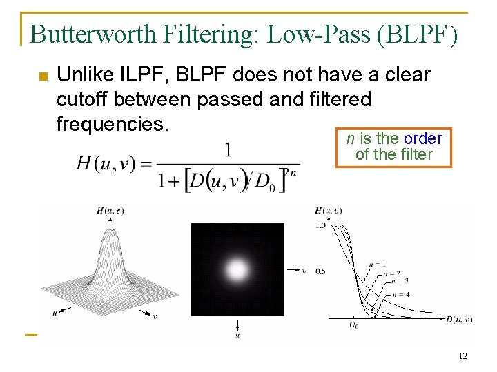
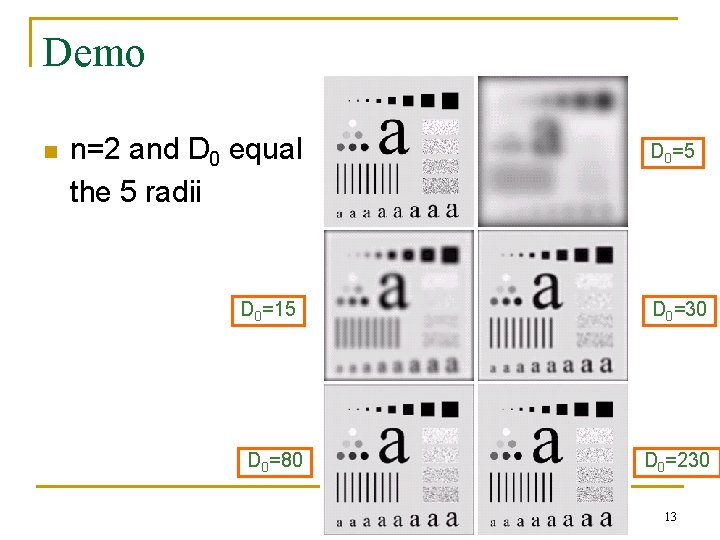
Butterworth Filtering: Low-Pass (BLPF) n Unlike ILPF, BLPF does not have a clear cutoff between passed and filtered frequencies. n is the order of the filter 12

Demo n n=2 and D 0 equal the 5 radii D 0=15 D 0=80 D 0=5 D 0=30 D 0=230 13

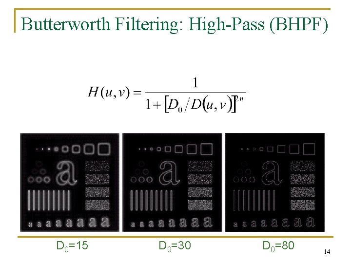
Butterworth Filtering: High-Pass (BHPF) D 0=15 D 0=30 D 0=80 14

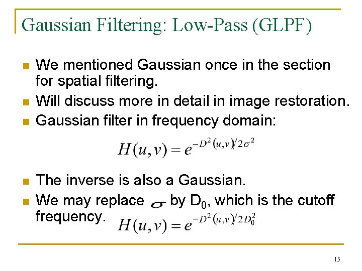
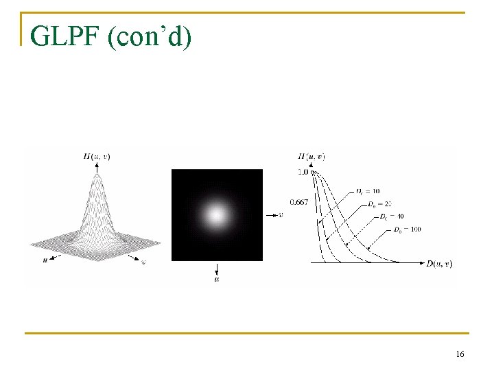
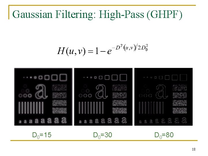
Gaussian Filtering: Low-Pass (GLPF) n n n We mentioned Gaussian once in the section for spatial filtering. Will discuss more in detail in image restoration. Gaussian filter in frequency domain: The inverse is also a Gaussian. We may replace by D 0, which is the cutoff frequency. 15

GLPF (con’d) 16

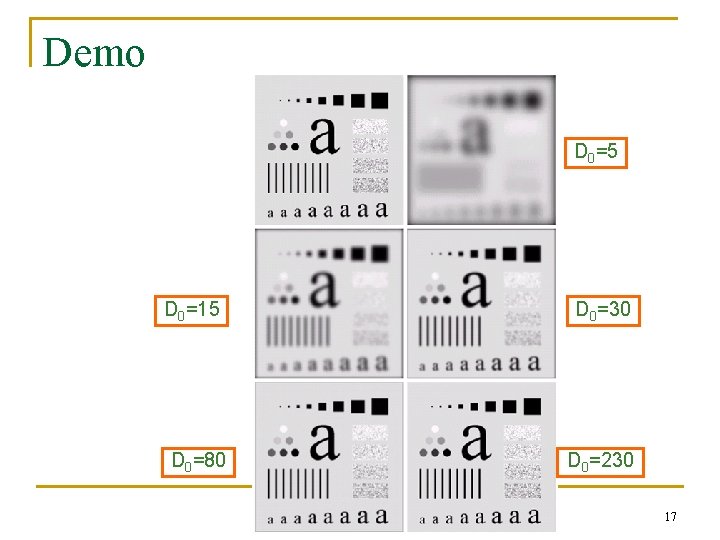
Demo D 0=5 D 0=15 D 0=80 D 0=30 D 0=230 17

Gaussian Filtering: High-Pass (GHPF) D 0=15 D 0=30 D 0=80 18

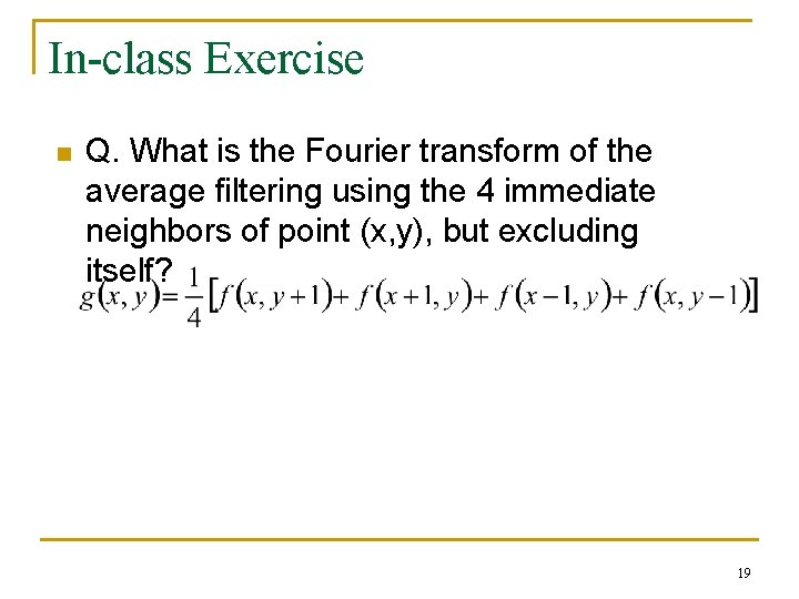
In-class Exercise n Q. What is the Fourier transform of the average filtering using the 4 immediate neighbors of point (x, y), but excluding itself? 19

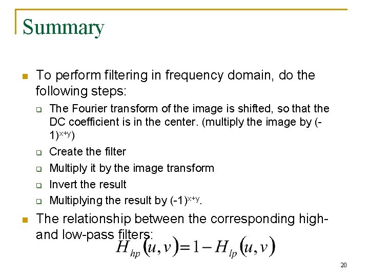
Summary n To perform filtering in frequency domain, do the following steps: q q q n The Fourier transform of the image is shifted, so that the DC coefficient is in the center. (multiply the image by (1)x+y) Create the filter Multiply it by the image transform Invert the result Multiplying the result by (-1)x+y. The relationship between the corresponding highand low-pass filters: 20

21