Digital Image Processing Image Enhancement Spatial Filtering 2

Digital Image Processing Image Enhancement (Spatial Filtering 2) Course Website: http: //www. comp. dit. ie/bmacnamee

2 of 39 Contents In this lecture we will look at more spatial filtering techniques – Spatial filtering refresher – Sharpening filters • 1 st derivative filters • 2 nd derivative filters – Combining filtering techniques

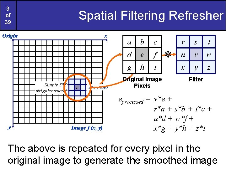
3 of 39 Spatial Filtering Refresher Origin x Simple 3*3 Neighbourhood y e 3*3 Filter Image f (x, y) a b c d e f g h i Original Image Pixels * r s t u v w x y z Filter eprocessed = v*e + r*a + s*b + t*c + u*d + w*f + x*g + y*h + z*i The above is repeated for every pixel in the original image to generate the smoothed image

4 of 39 Sharpening Spatial Filters Previously we have looked at smoothing filters which remove fine detail Sharpening spatial filters seek to highlight fine detail – Remove blurring from images – Highlight edges Sharpening filters are based on spatial differentiation

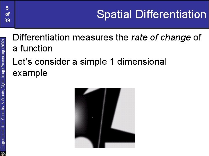
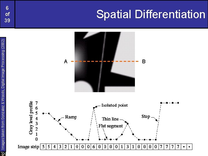
Images taken from Gonzalez & Woods, Digital Image Processing (2002) 5 of 39 Spatial Differentiation measures the rate of change of a function Let’s consider a simple 1 dimensional example

Images taken from Gonzalez & Woods, Digital Image Processing (2002) 6 of 39 Spatial Differentiation A B

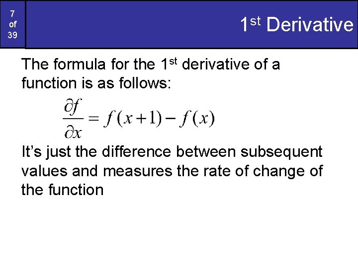
7 of 39 1 st Derivative The formula for the 1 st derivative of a function is as follows: It’s just the difference between subsequent values and measures the rate of change of the function

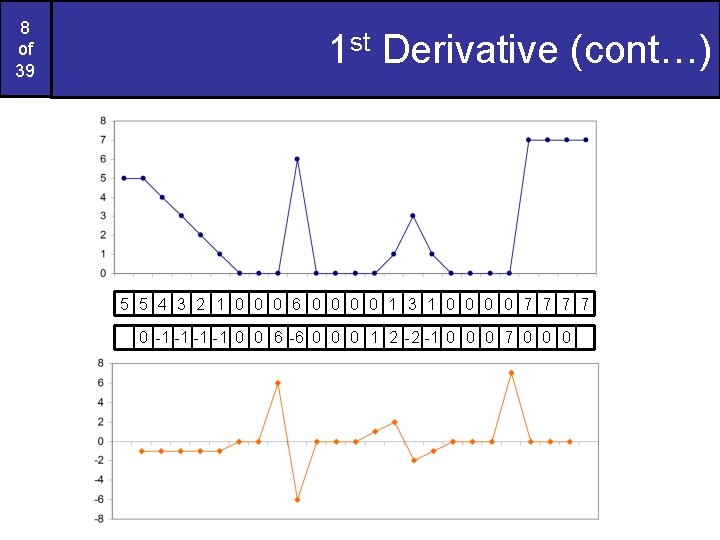
8 of 39 1 st Derivative (cont…) 5 5 4 3 2 1 0 0 0 6 0 0 1 3 1 0 0 7 7 0 -1 -1 0 0 6 -6 0 0 0 1 2 -2 -1 0 0 0 7 0 0 0

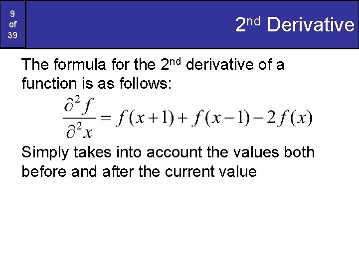
9 of 39 2 nd Derivative The formula for the 2 nd derivative of a function is as follows: Simply takes into account the values both before and after the current value

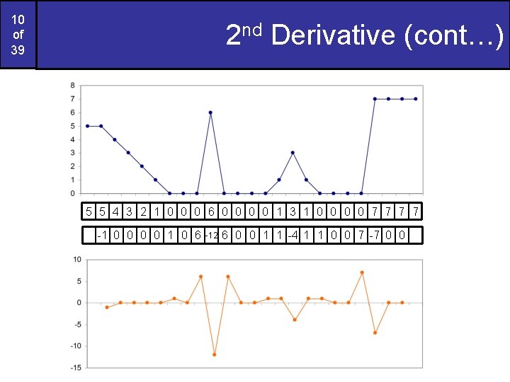
10 of 39 2 nd Derivative (cont…) 5 5 4 3 2 1 0 0 0 6 0 0 1 3 1 0 0 7 7 -1 0 0 1 0 6 -12 6 0 0 1 1 -4 1 1 0 0 7 -7 0 0

11 of 39 Using Second Derivatives For Image Enhancement The 2 nd derivative is more useful for image enhancement than the 1 st derivative – Stronger response to fine detail – Simpler implementation – We will come back to the 1 st order derivative later on The first sharpening filter we will look at is the Laplacian – Isotropic – One of the simplest sharpening filters – We will look at a digital implementation

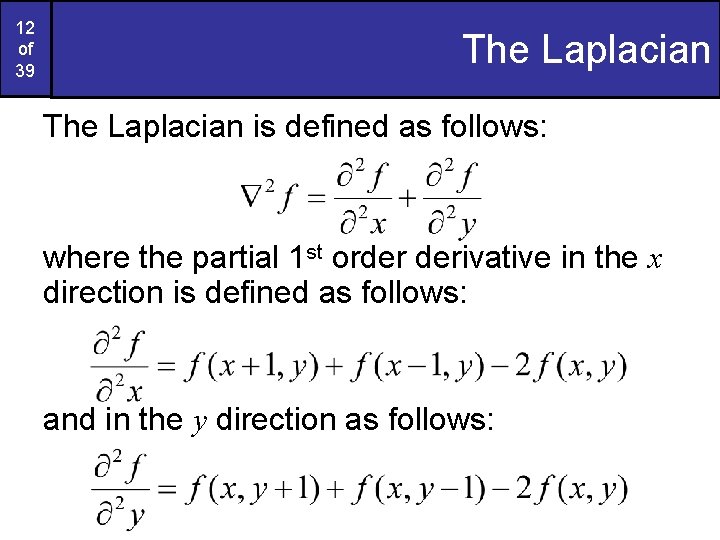
12 of 39 The Laplacian is defined as follows: where the partial 1 st order derivative in the x direction is defined as follows: and in the y direction as follows:

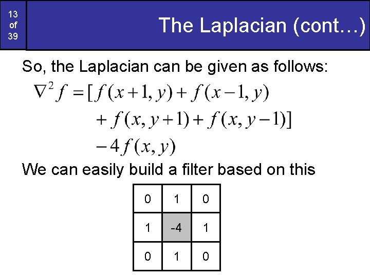
13 of 39 The Laplacian (cont…) So, the Laplacian can be given as follows: We can easily build a filter based on this 0 1 -4 1 0

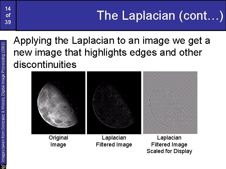
Images taken from Gonzalez & Woods, Digital Image Processing (2002) 14 of 39 The Laplacian (cont…) Applying the Laplacian to an image we get a new image that highlights edges and other discontinuities Original Image Laplacian Filtered Image Scaled for Display

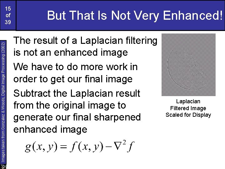
Images taken from Gonzalez & Woods, Digital Image Processing (2002) 15 of 39 But That Is Not Very Enhanced! The result of a Laplacian filtering is not an enhanced image We have to do more work in order to get our final image Subtract the Laplacian result from the original image to generate our final sharpened enhanced image Laplacian Filtered Image Scaled for Display

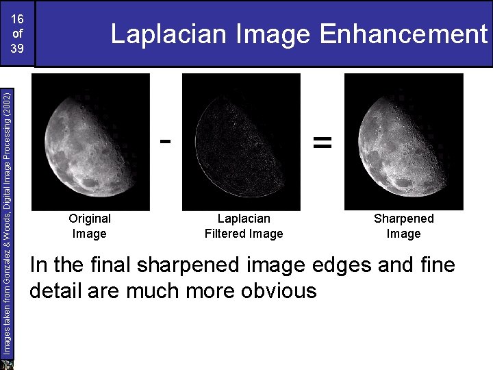
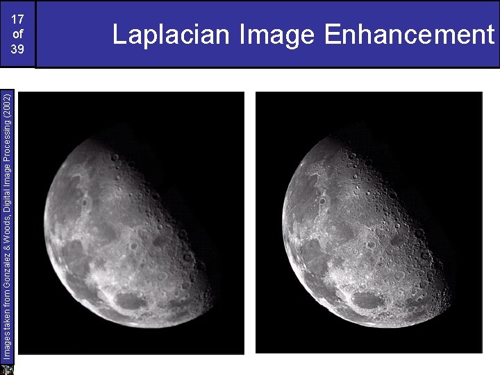
Images taken from Gonzalez & Woods, Digital Image Processing (2002) 16 of 39 Laplacian Image Enhancement Original Image = Laplacian Filtered Image Sharpened Image In the final sharpened image edges and fine detail are much more obvious

Images taken from Gonzalez & Woods, Digital Image Processing (2002) 17 of 39 Laplacian Image Enhancement

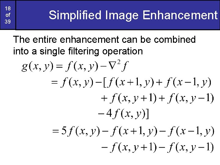
18 of 39 Simplified Image Enhancement The entire enhancement can be combined into a single filtering operation

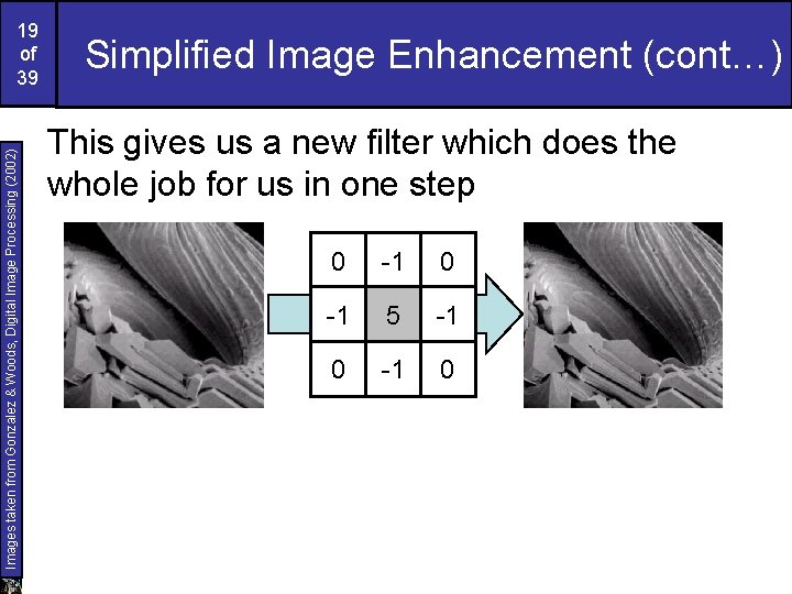
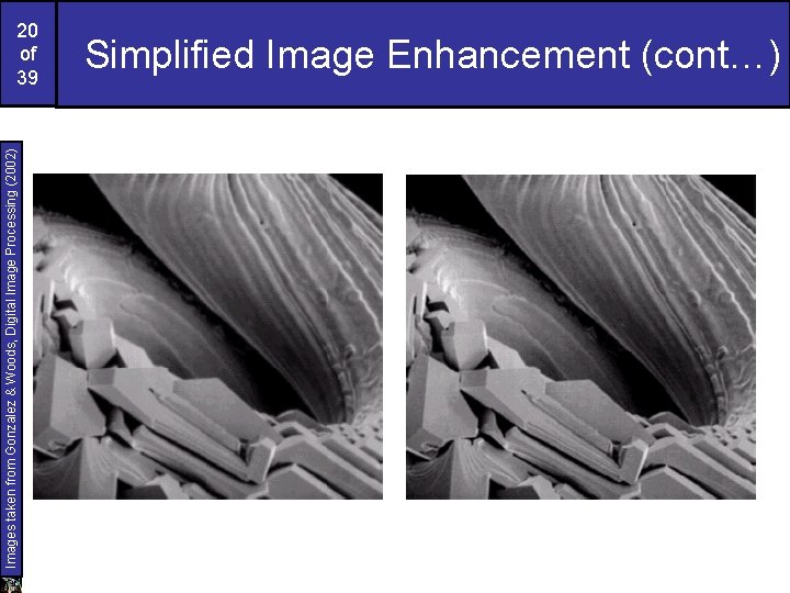
Images taken from Gonzalez & Woods, Digital Image Processing (2002) 19 of 39 Simplified Image Enhancement (cont…) This gives us a new filter which does the whole job for us in one step 0 -1 5 -1 0

Images taken from Gonzalez & Woods, Digital Image Processing (2002) 20 of 39 Simplified Image Enhancement (cont…)

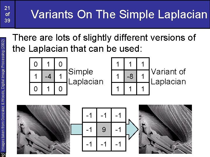
Images taken from Gonzalez & Woods, Digital Image Processing (2002) 21 of 39 Variants On The Simple Laplacian There are lots of slightly different versions of the Laplacian that can be used: 0 1 -4 1 0 Simple Laplacian 1 1 -8 1 1 -1 -1 9 -1 -1 Variant of Laplacian

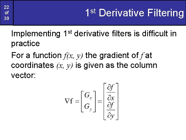
22 of 39 1 st Derivative Filtering Implementing 1 st derivative filters is difficult in practice For a function f(x, y) the gradient of f at coordinates (x, y) is given as the column vector:

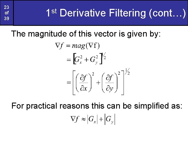
23 of 39 1 st Derivative Filtering (cont…) The magnitude of this vector is given by: For practical reasons this can be simplified as:

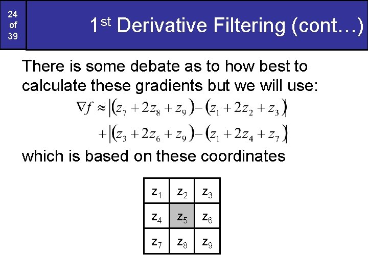
24 of 39 1 st Derivative Filtering (cont…) There is some debate as to how best to calculate these gradients but we will use: which is based on these coordinates z 1 z 2 z 3 z 4 z 5 z 6 z 7 z 8 z 9

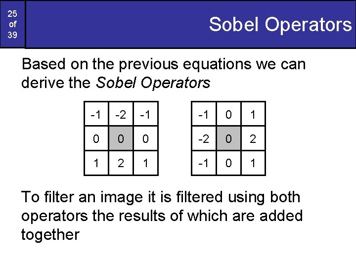
25 of 39 Sobel Operators Based on the previous equations we can derive the Sobel Operators -1 -2 -1 -1 0 0 0 -2 0 2 1 -1 0 1 To filter an image it is filtered using both operators the results of which are added together

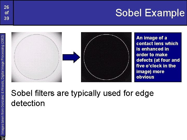
Images taken from Gonzalez & Woods, Digital Image Processing (2002) 26 of 39 Sobel Example An image of a contact lens which is enhanced in order to make defects (at four and five o’clock in the image) more obvious Sobel filters are typically used for edge detection

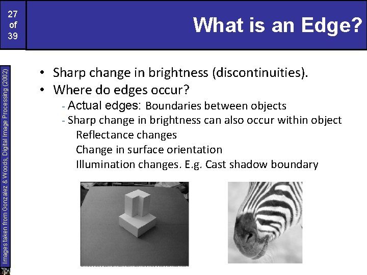
Images taken from Gonzalez & Woods, Digital Image Processing (2002) 27 of 39 What is an Edge? • Sharp change in brightness (discontinuities). • Where do edges occur? edges: Boundaries between objects - Sharp change in brightness can also occur within object Reflectance changes Change in surface orientation Illumination changes. E. g. Cast shadow boundary - Actual

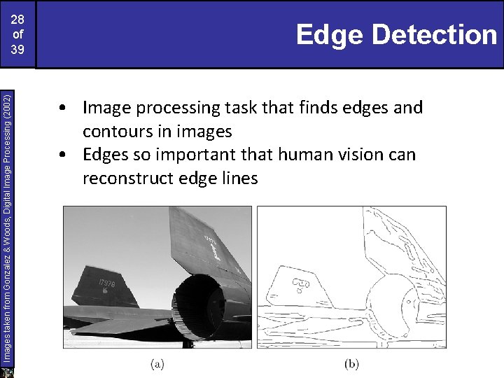
Images taken from Gonzalez & Woods, Digital Image Processing (2002) 28 of 39 Edge Detection • Image processing task that finds edges and contours in images • Edges so important that human vision can reconstruct edge lines

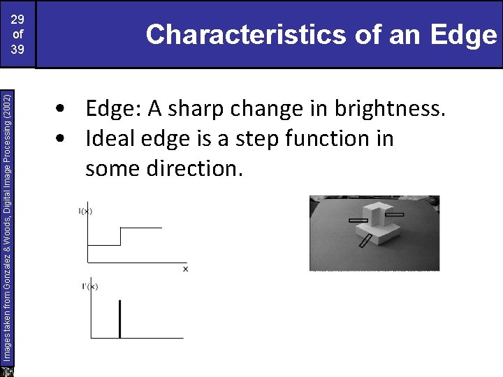
Images taken from Gonzalez & Woods, Digital Image Processing (2002) 29 of 39 Characteristics of an Edge • Edge: A sharp change in brightness. • Ideal edge is a step function in some direction.

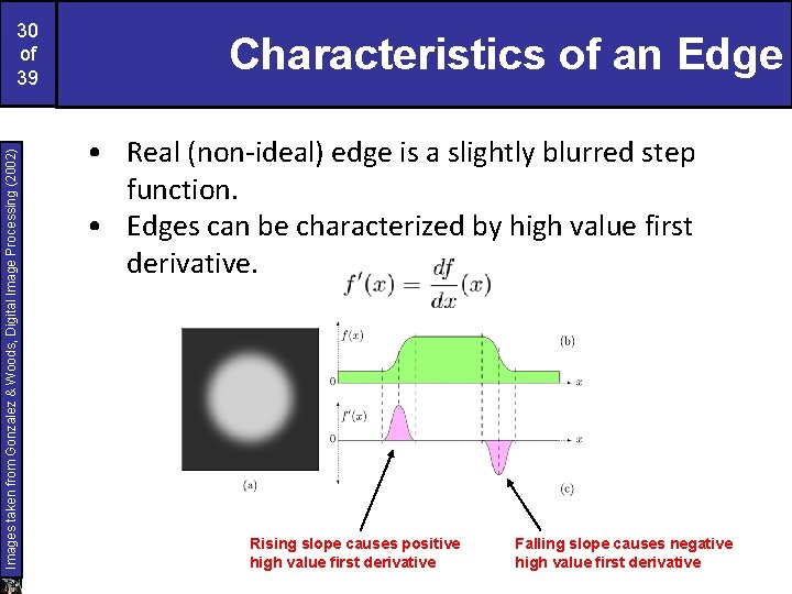
Images taken from Gonzalez & Woods, Digital Image Processing (2002) 30 of 39 Characteristics of an Edge • Real (non‐ideal) edge is a slightly blurred step function. • Edges can be characterized by high value first derivative. Rising slope causes positive high value first derivative Falling slope causes negative high value first derivative

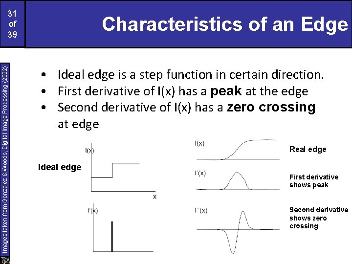
Images taken from Gonzalez & Woods, Digital Image Processing (2002) 31 of 39 Characteristics of an Edge • Ideal edge is a step function in certain direction. • First derivative of I(x) has a peak at the edge • Second derivative of I(x) has a zero crossing at edge Real edge Ideal edge First derivative shows peak Second derivative shows zero crossing

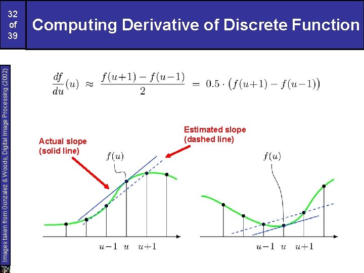
Images taken from Gonzalez & Woods, Digital Image Processing (2002) 32 of 39 Computing Derivative of Discrete Function Actual slope (solid line) Estimated slope (dashed line)

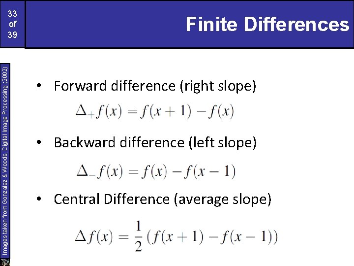
Images taken from Gonzalez & Woods, Digital Image Processing (2002) 33 of 39 Finite Differences • Forward difference (right slope) • Backward difference (left slope) • Central Difference (average slope)

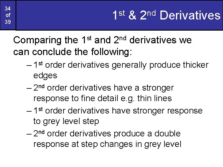
34 of 39 1 st & 2 nd Derivatives Comparing the 1 st and 2 nd derivatives we can conclude the following: – 1 st order derivatives generally produce thicker edges – 2 nd order derivatives have a stronger response to fine detail e. g. thin lines – 1 st order derivatives have stronger response to grey level step – 2 nd order derivatives produce a double response at step changes in grey level

35 of 39 Summary In this lecture we looked at: – Sharpening filters • 1 st derivative filters • 2 nd derivative filters – Combining filtering techniques

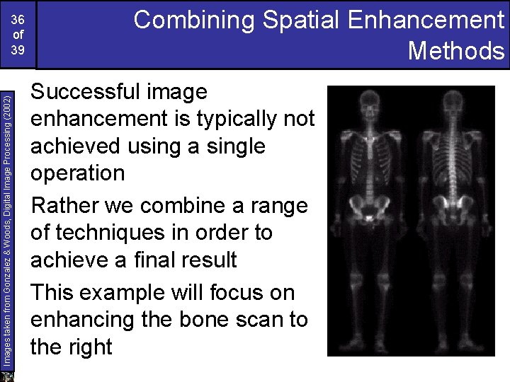
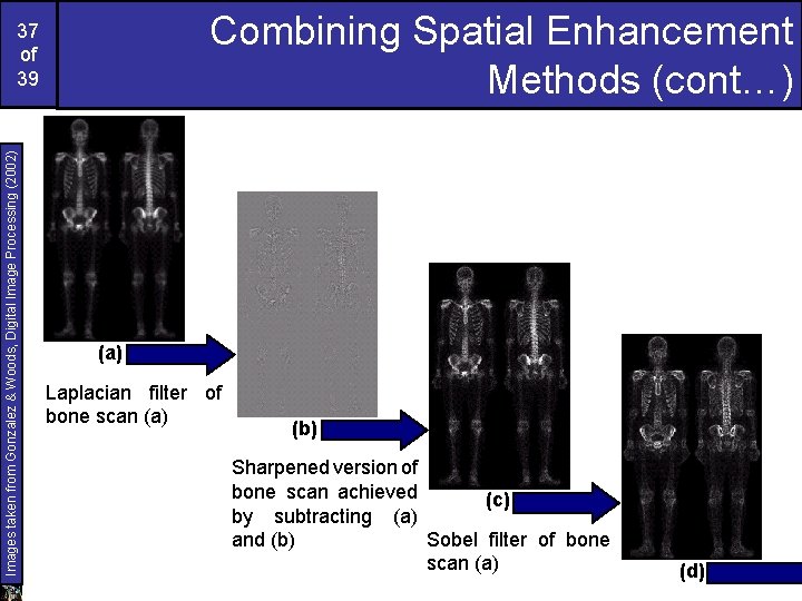
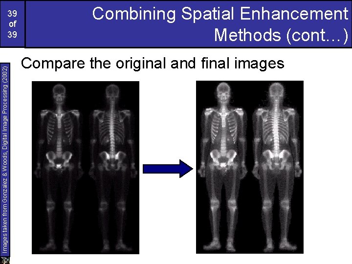
Images taken from Gonzalez & Woods, Digital Image Processing (2002) 36 of 39 Combining Spatial Enhancement Methods Successful image enhancement is typically not achieved using a single operation Rather we combine a range of techniques in order to achieve a final result This example will focus on enhancing the bone scan to the right

Combining Spatial Enhancement Methods (cont…) Images taken from Gonzalez & Woods, Digital Image Processing (2002) 37 of 39 (a) Laplacian filter of bone scan (a) (b) Sharpened version of bone scan achieved (c) by subtracting (a) Sobel filter of bone and (b) scan (a) (d)

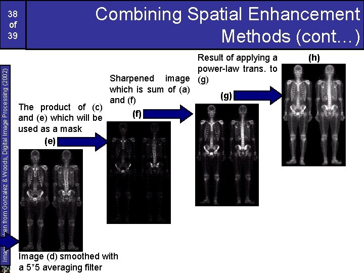
Images taken from Gonzalez & Woods, Digital Image Processing (2002) 38 of 39 Combining Spatial Enhancement Methods (cont…) The product of (c) and (e) which will be used as a mask (e) Result of applying a power-law trans. to Sharpened image (g) which is sum of (a) (g) and (f) Image (d) smoothed with a 5*5 averaging filter (f) (h)

Images taken from Gonzalez & Woods, Digital Image Processing (2002) 39 of 39 Combining Spatial Enhancement Methods (cont…) Compare the original and final images