CSE 5311 Design and Analysis of Algorithms Administrivia

CSE 5311 Design and Analysis of Algorithms Administrivia Introduction Review of Basics 1/5/2022 CSE 5311 SPRING 2004 MKUMAR 1

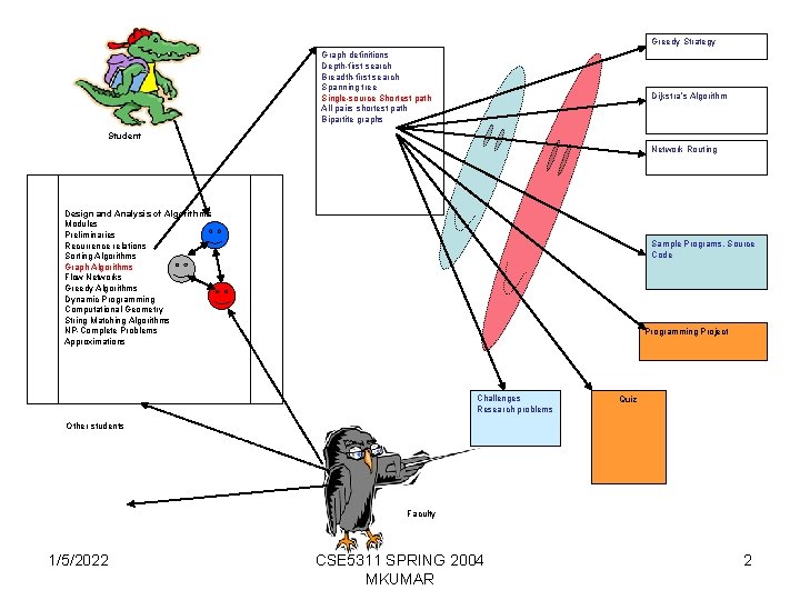
Greedy Strategy Graph definitions Depth-first search Breadth-first search Spanning tree Single-source Shortest path All-pairs shortest path Bipartite graphs Dijkstra’s Algorithm Student Network Routing Design and Analysis of Algorithms Modules Preliminaries Recurrence relations Sorting Algorithms Graph Algorithms Flow Networks Greedy Algorithms Dynamic Programming Computational Geometry String Matching Algorithms NP-Complete Problems Approximations Sample Programs, Source Code Programming Project Challenges Research problems Quiz Other students Faculty 1/5/2022 CSE 5311 SPRING 2004 MKUMAR 2

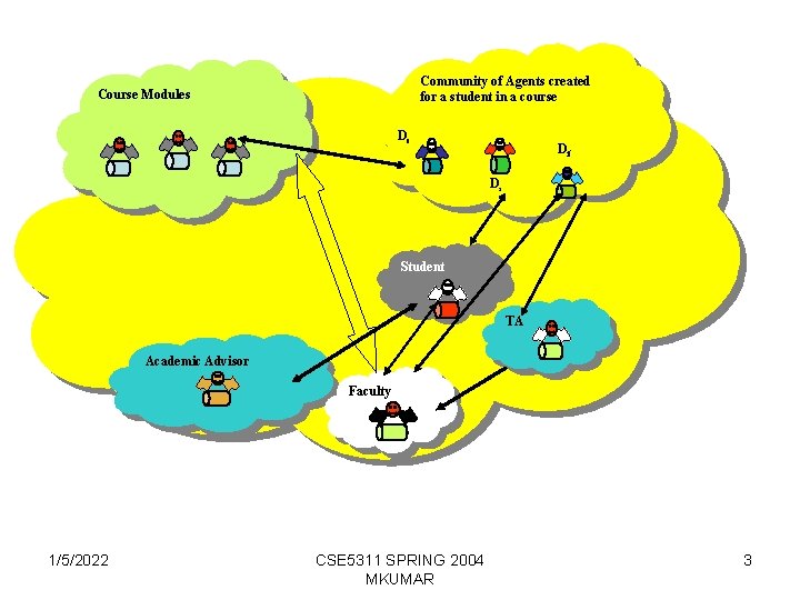
Community of Agents created for a student in a course Course Modules Dc Df Ds Student TA Academic Advisor Faculty 1/5/2022 CSE 5311 SPRING 2004 MKUMAR 3

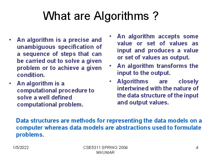
What are Algorithms ? • An algorithm is a precise and unambiguous specification of a sequence of steps that can be carried out to solve a given problem or to achieve a given condition. • An algorithm is a computational procedure to solve a well defined computational problem. • An algorithm accepts some value or set of values as input and produces a value or set of values as output. • An algorithm transforms the input to the output. • Algorithms are closely intertwined with the nature of the data structure of the input and output values. Data structures are methods for representing the data models on a computer whereas data models are abstractions used to formulate problems. 1/5/2022 CSE 5311 SPRING 2004 MKUMAR 4

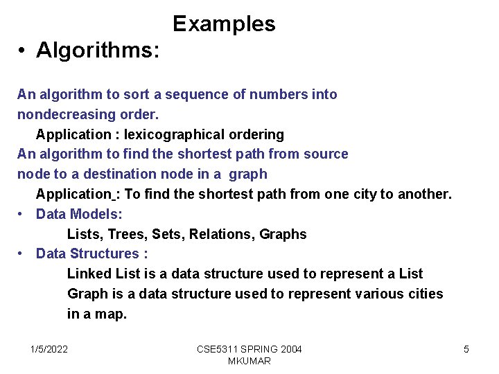
Examples • Algorithms: An algorithm to sort a sequence of numbers into nondecreasing order. Application : lexicographical ordering An algorithm to find the shortest path from source node to a destination node in a graph Application : To find the shortest path from one city to another. • Data Models: Lists, Trees, Sets, Relations, Graphs • Data Structures : Linked List is a data structure used to represent a List Graph is a data structure used to represent various cities in a map. 1/5/2022 CSE 5311 SPRING 2004 MKUMAR 5

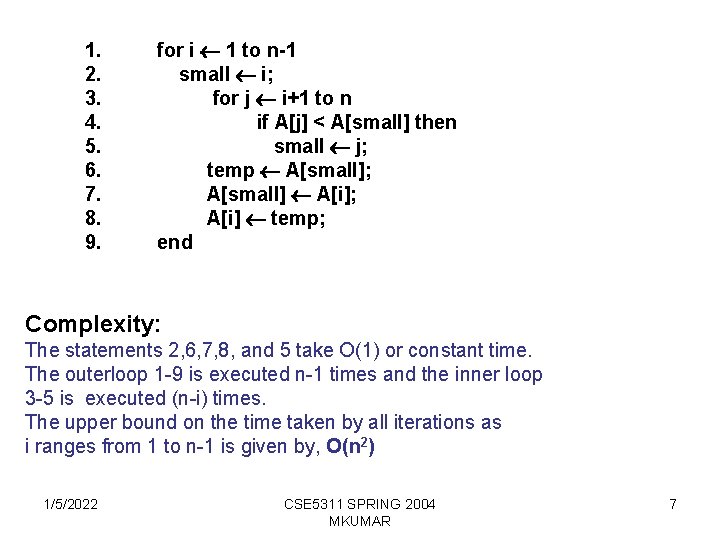
SELECTION SORT Algorithm (Iterative method) Procedure SELECTION_SORT (A [1, …, n]) Input : unsorted array A Output : Sorted array A 1. 2. 3. 4. 5. 6. 7. 8. 9. for i 1 to n-1 small i; for j i+1 to n if A[j] < A[small] then small j; Example : Given sequence temp A[small]; 5 2 4 6 1 3 A[small] A[i]; i=1 1 2 4 6 5 3 A[i] temp; i=2 1 2 4 6 5 3 end 1/5/2022 i=3 i=4 CSE 5311 SPRING 2004 MKUMAR 1 1 2 2 3 3 6 4 5 5 4 6 6

1. 2. 3. 4. 5. 6. 7. 8. 9. for i 1 to n-1 small i; for j i+1 to n if A[j] < A[small] then small j; temp A[small]; A[small] A[i]; A[i] temp; end Complexity: The statements 2, 6, 7, 8, and 5 take O(1) or constant time. The outerloop 1 -9 is executed n-1 times and the inner loop 3 -5 is executed (n-i) times. The upper bound on the time taken by all iterations as i ranges from 1 to n-1 is given by, O(n 2) 1/5/2022 CSE 5311 SPRING 2004 MKUMAR 7

• Study of algorithms involves, Ødesigning algorithms Øexpressing algorithms Øalgorithm validation Øalgorithm analysis ØStudy of algorithmic techniques 1/5/2022 CSE 5311 SPRING 2004 MKUMAR 8

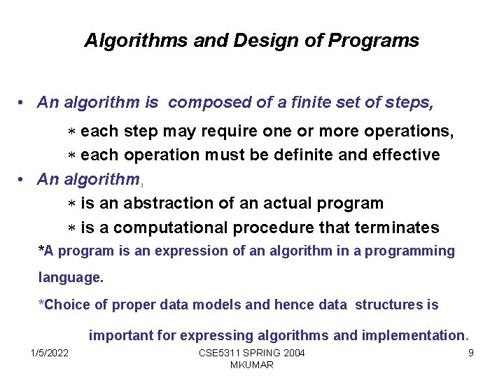
Algorithms and Design of Programs • An algorithm is composed of a finite set of steps, * each step may require one or more operations, * each operation must be definite and effective • An algorithm, * is an abstraction of an actual program * is a computational procedure that terminates *A program is an expression of an algorithm in a programming language. *Choice of proper data models and hence data structures is important for expressing algorithms and implementation. 1/5/2022 CSE 5311 SPRING 2004 MKUMAR 9

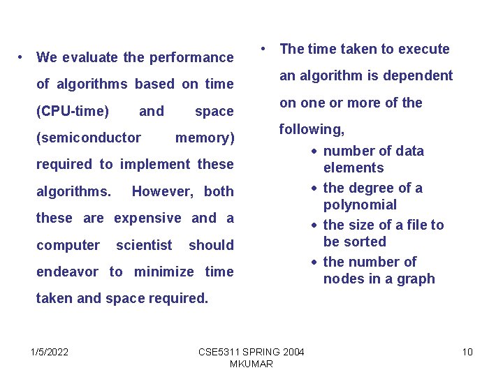
• We evaluate the performance of algorithms based on time (CPU-time) and (semiconductor space memory) • The time taken to execute an algorithm is dependent on one or more of the following, required to implement these algorithms. However, both these are expensive and a computer scientist should endeavor to minimize time · number of data elements · the degree of a polynomial · the size of a file to be sorted · the number of nodes in a graph taken and space required. 1/5/2022 CSE 5311 SPRING 2004 MKUMAR 10

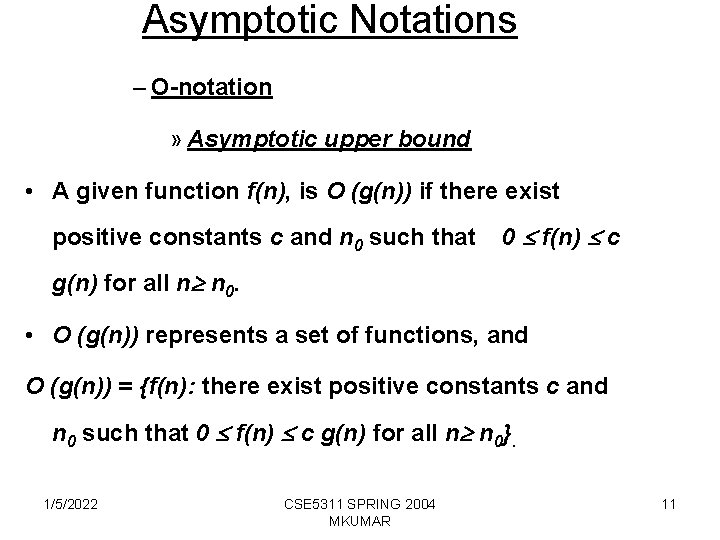
Asymptotic Notations – O-notation » Asymptotic upper bound • A given function f(n), is O (g(n)) if there exist positive constants c and n 0 such that 0 f(n) c g(n) for all n n 0. • O (g(n)) represents a set of functions, and O (g(n)) = {f(n): there exist positive constants c and n 0 such that 0 f(n) c g(n) for all n n 0}. 1/5/2022 CSE 5311 SPRING 2004 MKUMAR 11

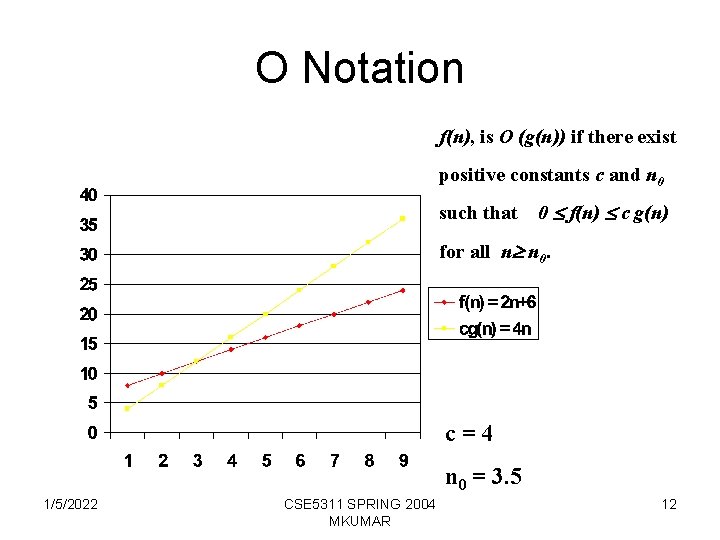
O Notation f(n), is O (g(n)) if there exist positive constants c and n 0 such that 0 f(n) c g(n) for all n n 0. c=4 n 0 = 3. 5 1/5/2022 CSE 5311 SPRING 2004 MKUMAR 12

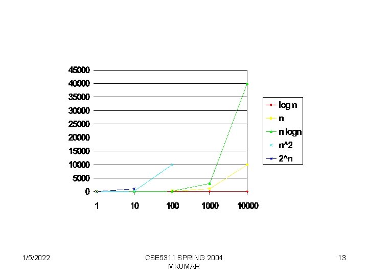
1/5/2022 CSE 5311 SPRING 2004 MKUMAR 13

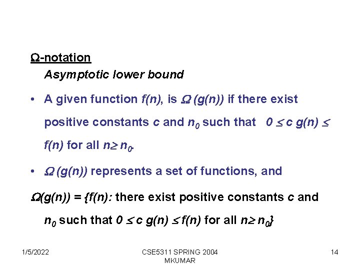
-notation Asymptotic lower bound • A given function f(n), is (g(n)) if there exist positive constants c and n 0 such that 0 c g(n) f(n) for all n n 0. • (g(n)) represents a set of functions, and (g(n)) = {f(n): there exist positive constants c and n 0 such that 0 c g(n) f(n) for all n n 0} 1/5/2022 CSE 5311 SPRING 2004 MKUMAR 14

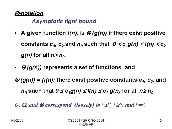
-notation Asymptotic tight bound • A given function f(n), is (g(n)) if there exist positive constants c 1, c 2, and n 0 such that 0 c 1 g(n) f(n) c 2 g(n) for all n n 0. • (g(n)) represents a set of functions, and (g(n)) = {f(n): there exist positive constants c 1, c 2, and n 0 such that 0 c 1 g(n) f(n) c 2 g(n) for all n n 0. O, , and correspond (loosely) to “ ”, and “=”. 1/5/2022 CSE 5311 SPRING 2004 MKUMAR 15

Presenting algorithms • Description : The algorithm will be described in English, with the help of one or more examples • Specification : The algorithm will be presented as pseudocode (We don't use any programming language) • Validation : The algorithm will be proved to be correct for all problem cases • Analysis: The running time or time complexity of the algorithm will be evaluated 1/5/2022 CSE 5311 SPRING 2004 MKUMAR 16

SELECTION SORT Algorithm (Iterative method) Procedure SELECTION_SORT (A [1, …, n]) Input : unsorted array A Output : Sorted array A 1. 2. 3. 4. 5. 6. 7. 8. 9. 1/5/2022 for i 1 to n-1 small i; for j i+1 to n if A[j] < A[small] then small j; temp A[small]; A[small] A[i]; A[i] temp; end CSE 5311 SPRING 2004 MKUMAR 17

Recursive Selection Sort Algorithm Given an array A[i, …, n], selection sort picks the smallest element in the array and swaps it with A[i], then sorts the remainder A[i+1, …, n] recursively. Example : Given A [26, 93, 36, 76, 85, 09, 42, 64] Swap 09 with 23, A[1] = 09, A[2, …, 8] = [93, 36, 76, 85, 26, 42, 64] Swap 26 with 93, A[1, 2]= [09, 26]; A[3, …, 8] = [36, 76, 85, 93, 42, 64] No swapping A[1, 2, 3] = [09, 26, 36]; A[4, …, 8] =[76, 85, 93, 42, 64] Swap 42 with 76, A[1, …, 4] =[09, 26, 36, 42]; A[5, …, 8] = [85, 93, 76, 64] Swap 64 with 85, A[1, …, 5] =[09, 26, 36, 42, 64]; A[6, 7, 8] = [93, 76, 85] Swap 76 with 93, A[1, …, 6]=[09, 26, 36, 42, 64, 76]; A[7, 8] = [93, 85] Swap 85 with 93, A[1, …, 7]=[09, 26, 36, 42, 64, 76, 85]; A[8] = 93 Sorted list : A[1, …, 8] = [09, 26, 36, 42, 64, 76, 85, 93] 1/5/2022 CSE 5311 SPRING 2004 MKUMAR 18

Procedure RECURSIVE_SELECTION_SORT (A[1, …, n], i, n) Input : Unsorted array A Output : Sorted array A while i < n do small i; for j i+1 to n if A[j] < A[small] then small j; temp A[small]; A[small] A[i]; A[i] temp; RECURSIVE_SELECTION_SORT(A, i+1, n) End 1/5/2022 CSE 5311 SPRING 2004 MKUMAR 19

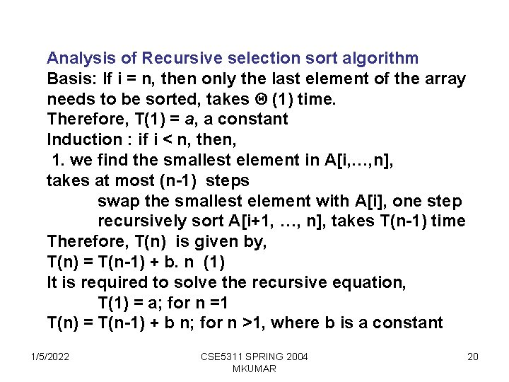
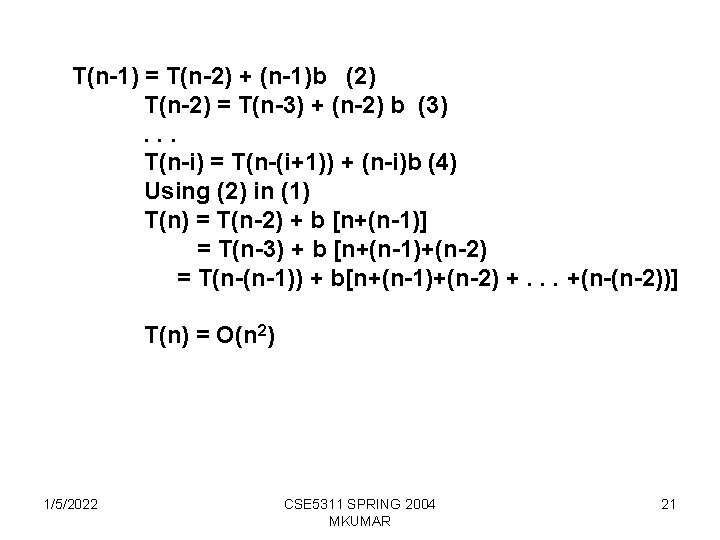
Analysis of Recursive selection sort algorithm Basis: If i = n, then only the last element of the array needs to be sorted, takes (1) time. Therefore, T(1) = a, a constant Induction : if i < n, then, 1. we find the smallest element in A[i, …, n], takes at most (n-1) steps swap the smallest element with A[i], one step recursively sort A[i+1, …, n], takes T(n-1) time Therefore, T(n) is given by, T(n) = T(n-1) + b. n (1) It is required to solve the recursive equation, T(1) = a; for n =1 T(n) = T(n-1) + b n; for n >1, where b is a constant 1/5/2022 CSE 5311 SPRING 2004 MKUMAR 20

T(n-1) = T(n-2) + (n-1)b (2) T(n-2) = T(n-3) + (n-2) b (3). . . T(n-i) = T(n-(i+1)) + (n-i)b (4) Using (2) in (1) T(n) = T(n-2) + b [n+(n-1)] = T(n-3) + b [n+(n-1)+(n-2) = T(n-(n-1)) + b[n+(n-1)+(n-2) +. . . +(n-(n-2))] T(n) = O(n 2) 1/5/2022 CSE 5311 SPRING 2004 MKUMAR 21

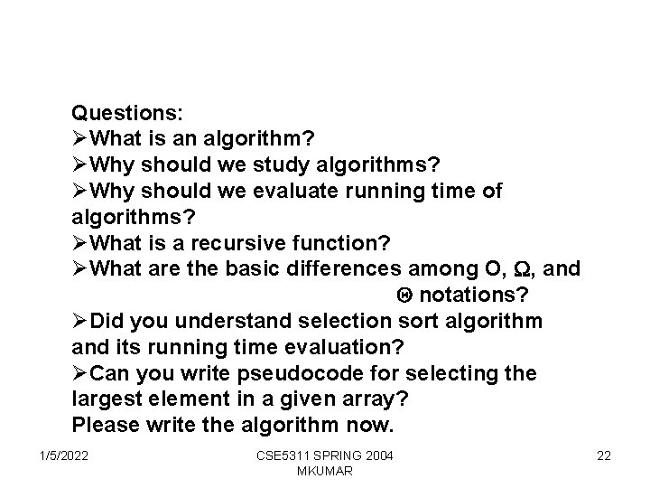
Questions: ØWhat is an algorithm? ØWhy should we study algorithms? ØWhy should we evaluate running time of algorithms? ØWhat is a recursive function? ØWhat are the basic differences among O, , and notations? ØDid you understand selection sort algorithm and its running time evaluation? ØCan you write pseudocode for selecting the largest element in a given array? Please write the algorithm now. 1/5/2022 CSE 5311 SPRING 2004 MKUMAR 22

Heaps and Heapsort Further Reading Chapters 6 from Textbook This week q. Priority Trees q. Building Heaps q. Maintaining heaps q. Heapsort Algorithm q. Analysis of Heapsort Algorithm 1/5/2022 CSE 5311 SPRING 2004 MKUMAR 23

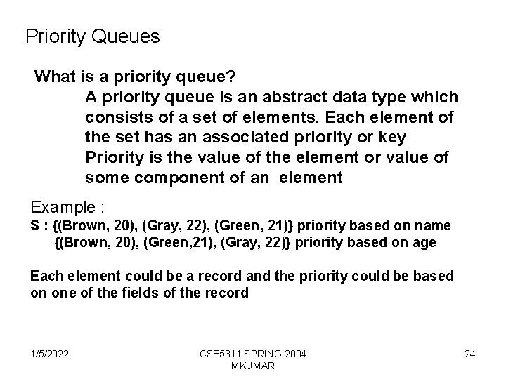
Priority Queues What is a priority queue? A priority queue is an abstract data type which consists of a set of elements. Each element of the set has an associated priority or key Priority is the value of the element or value of some component of an element Example : S : {(Brown, 20), (Gray, 22), (Green, 21)} priority based on name {(Brown, 20), (Green, 21), (Gray, 22)} priority based on age Each element could be a record and the priority could be based on one of the fields of the record 1/5/2022 CSE 5311 SPRING 2004 MKUMAR 24

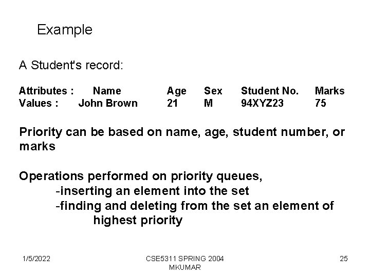
Example A Student's record: Attributes : Name Values : John Brown Age 21 Sex M Student No. 94 XYZ 23 Marks 75 Priority can be based on name, age, student number, or marks Operations performed on priority queues, -inserting an element into the set -finding and deleting from the set an element of highest priority 1/5/2022 CSE 5311 SPRING 2004 MKUMAR 25

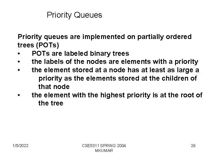
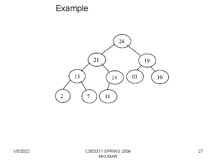
Priority Queues Priority queues are implemented on partially ordered trees (POTs) • POTs are labeled binary trees • the labels of the nodes are elements with a priority • the element stored at a node has at least as large a priority as the elements stored at the children of that node • the element with the highest priority is at the root of the tree 1/5/2022 CSE 5311 SPRING 2004 MKUMAR 26

Example 1/5/2022 CSE 5311 SPRING 2004 MKUMAR 27

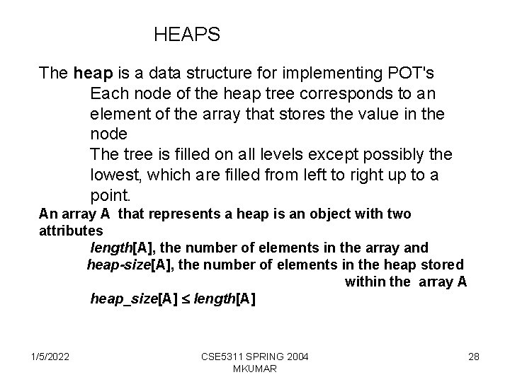
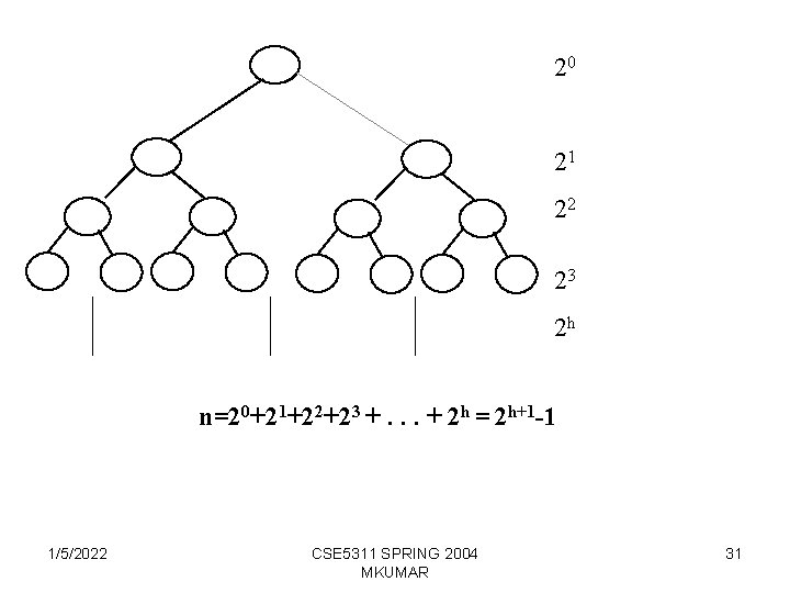
HEAPS The heap is a data structure for implementing POT's Each node of the heap tree corresponds to an element of the array that stores the value in the node The tree is filled on all levels except possibly the lowest, which are filled from left to right up to a point. An array A that represents a heap is an object with two attributes length[A], the number of elements in the array and heap-size[A], the number of elements in the heap stored within the array A heap_size[A] length[A] 1/5/2022 CSE 5311 SPRING 2004 MKUMAR 28

HEAPS (Contd) The heap comprises elements in locations up to heap-size[A]. A[1] is the root of the tree. Position 1 Value 24 2 3 4 5 6 7 8 9 10 21 19 13 14 3 10 2 7 11 Given node with index i, PARENT(i) is the index of parent of i; PARENT(i) = i/2 LEFT_CHILD(i) is the index of left child of i ; LEFT_CHILD(i) = 2 i; RIGHT_CHILD(i) is the index of right child of i; and RIGHT_CHILD(i) = 2 i +1 1/5/2022 CSE 5311 SPRING 2004 MKUMAR 29

Heap Property THE HEAP PROPERTY A[PARENT(i)] A[i] The heap is based on a binary tree The height of the heap (as a binary tree) is the number of edges on the longest simple downward path from the root to a leaf. The height of a heap with n nodes is O (log n). All basic operations on heaps run in O (log n) time. 1/5/2022 CSE 5311 SPRING 2004 MKUMAR 30

20 21 22 23 2 h n=20+21+22+23 +. . . + 2 h = 2 h+1 -1 1/5/2022 CSE 5311 SPRING 2004 MKUMAR 31

Heap Algorithms HEAPIFY BUILD_HEAPSORT HEAP_EXTRACT_MAX HEAP_INSERT 1/5/2022 CSE 5311 SPRING 2004 MKUMAR 32

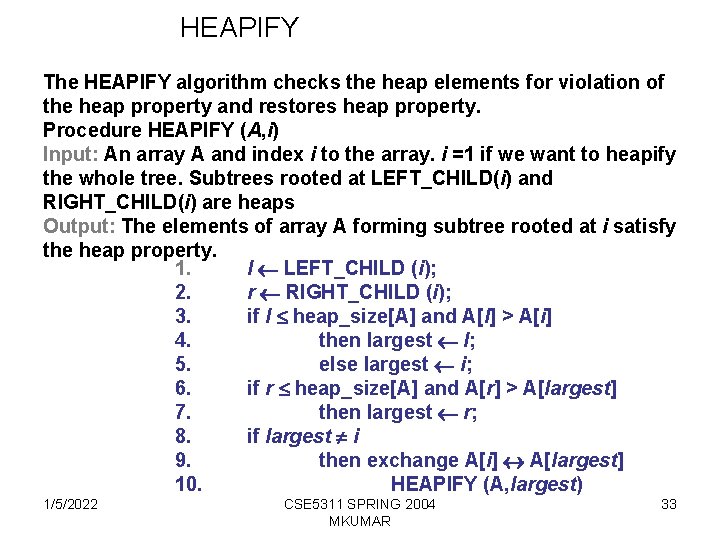
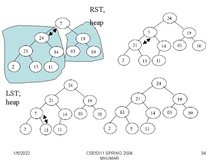
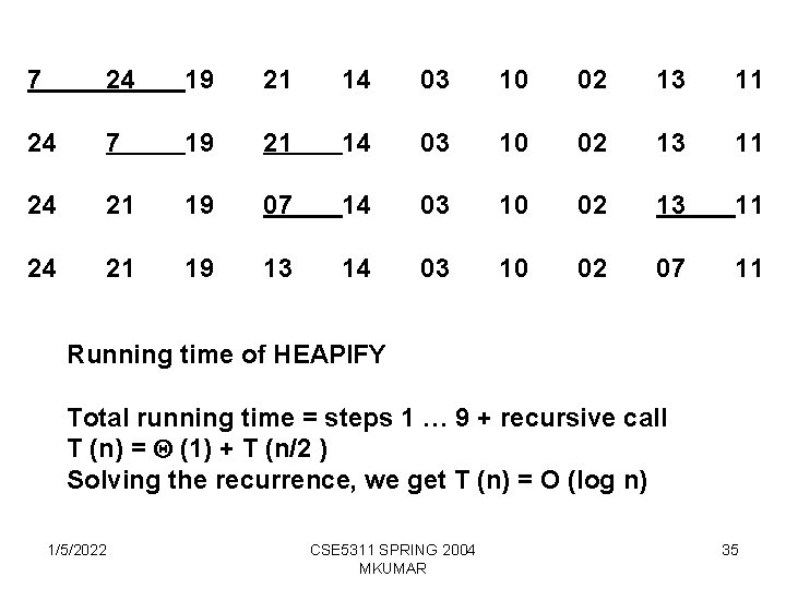
HEAPIFY The HEAPIFY algorithm checks the heap elements for violation of the heap property and restores heap property. Procedure HEAPIFY (A, i) Input: An array A and index i to the array. i =1 if we want to heapify the whole tree. Subtrees rooted at LEFT_CHILD(i) and RIGHT_CHILD(i) are heaps Output: The elements of array A forming subtree rooted at i satisfy the heap property. 1. l LEFT_CHILD (i); 2. r RIGHT_CHILD (i); 3. if l heap_size[A] and A[l] > A[i] 4. then largest l; 5. else largest i; 6. if r heap_size[A] and A[r] > A[largest] 7. then largest r; 8. if largest i 9. then exchange A[i] A[largest] 10. HEAPIFY (A, largest) 1/5/2022 CSE 5311 SPRING 2004 MKUMAR 33

RST, heap LST; heap 1/5/2022 CSE 5311 SPRING 2004 MKUMAR 34

7 24 19 21 14 03 10 02 13 11 24 7 19 21 14 03 10 02 13 11 24 21 19 07 14 03 10 02 13 11 24 21 19 13 14 03 10 02 07 11 Running time of HEAPIFY Total running time = steps 1 … 9 + recursive call T (n) = (1) + T (n/2 ) Solving the recurrence, we get T (n) = O (log n) 1/5/2022 CSE 5311 SPRING 2004 MKUMAR 35

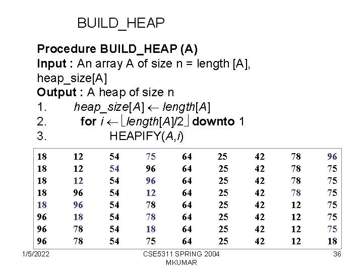
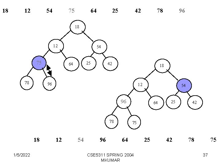
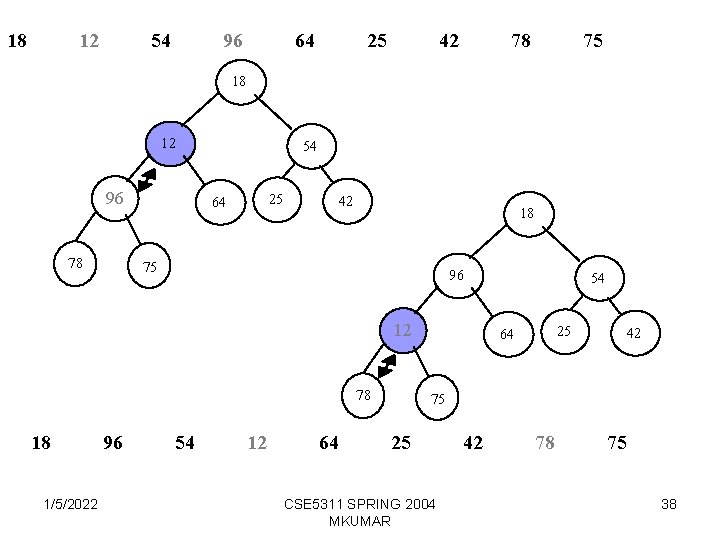
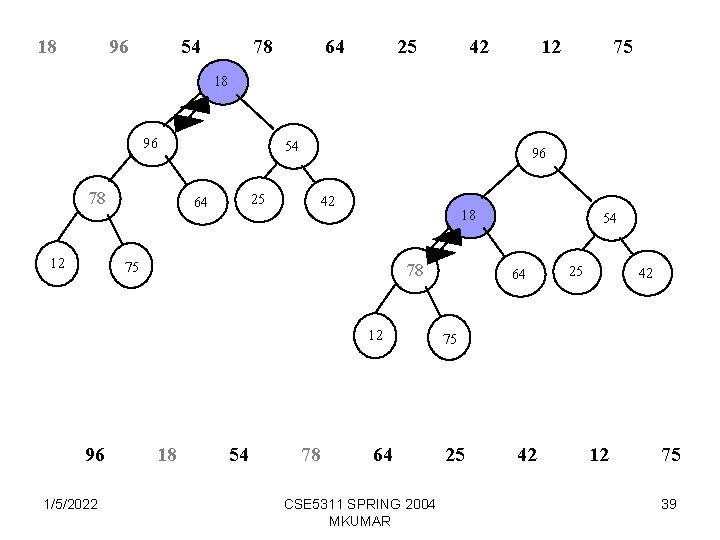
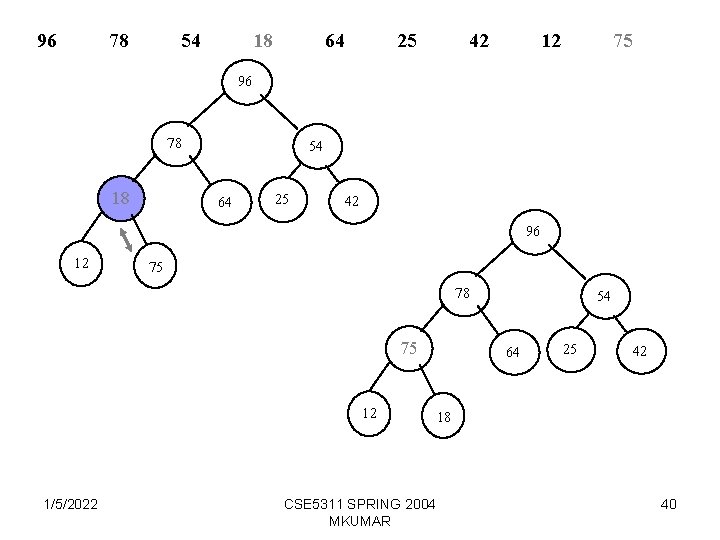
BUILD_HEAP Procedure BUILD_HEAP (A) Input : An array A of size n = length [A], heap_size[A] Output : A heap of size n 1. heap_size[A] length[A] 2. for i length[A]/2 downto 1 3. HEAPIFY(A, i) 18 18 18 96 96 96 1/5/2022 12 12 12 96 96 18 78 78 54 54 75 96 96 12 78 78 18 75 64 64 25 25 CSE 5311 SPRING 2004 MKUMAR 42 42 78 78 12 12 96 75 75 75 18 36

18 12 54 75 64 25 42 78 96 18 12 75 78 54 25 64 42 18 96 12 54 96 78 18 1/5/2022 12 54 96 64 25 42 75 64 CSE 5311 SPRING 2004 MKUMAR 25 42 78 75 37

18 12 54 96 64 25 42 78 75 18 12 96 78 54 25 64 42 18 75 96 12 78 18 1/5/2022 96 54 12 64 54 25 64 42 75 25 CSE 5311 SPRING 2004 MKUMAR 42 78 75 38

18 96 54 78 64 25 42 12 75 18 96 78 12 54 25 64 96 42 18 75 78 12 96 1/5/2022 18 54 78 64 CSE 5311 SPRING 2004 MKUMAR 54 64 25 42 75 25 42 12 75 39

96 78 54 18 64 25 42 12 75 96 78 18 54 64 25 42 96 12 75 78 75 12 1/5/2022 CSE 5311 SPRING 2004 MKUMAR 54 64 25 42 18 40

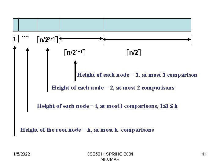
1 n/22+1 n/21+1 n/2 Height of each node = 1, at most 1 comparison Height of each node = 2, at most 2 comparisons Height of each node = i, at most i comparisons, 1 i h Height of the root node = h, at most h comparisons 1/5/2022 CSE 5311 SPRING 2004 MKUMAR 41

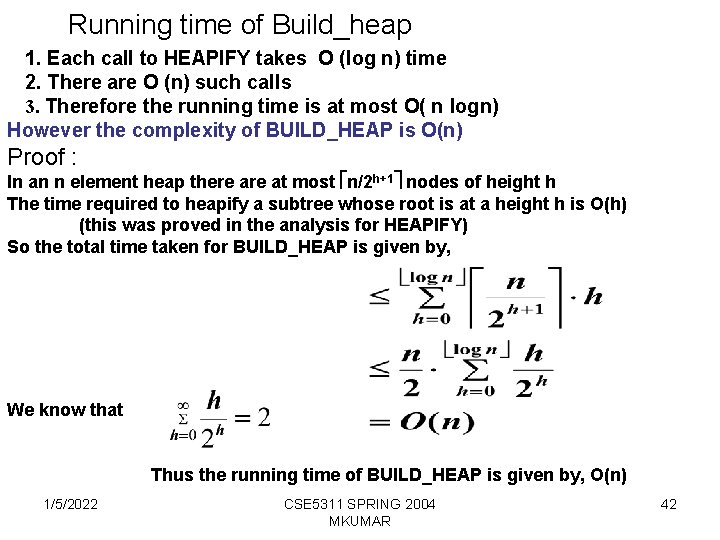
Running time of Build_heap 1. Each call to HEAPIFY takes O (log n) time 2. There are O (n) such calls 3. Therefore the running time is at most O( n logn) However the complexity of BUILD_HEAP is O(n) Proof : In an n element heap there at most n/2 h+1 nodes of height h The time required to heapify a subtree whose root is at a height h is O(h) (this was proved in the analysis for HEAPIFY) So the total time taken for BUILD_HEAP is given by, We know that Thus the running time of BUILD_HEAP is given by, O(n) 1/5/2022 CSE 5311 SPRING 2004 MKUMAR 42

The HEAPSORT Algorithm Procedure HEAPSORT(A) Input : Array A[1…n], n = length[A] Output : Sorted array A[1…n] 1. BUILD_HEAP[A] 2. for i length[A] down to 2 3. Exchange A[1] A[i] 4. heap_size[A]-1; 5. HEAPIFY(A, 1) Example : To be given in the lecture 1/5/2022 CSE 5311 SPRING 2004 MKUMAR 43

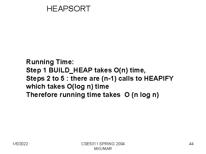
HEAPSORT Running Time: Step 1 BUILD_HEAP takes O(n) time, Steps 2 to 5 : there are (n-1) calls to HEAPIFY which takes O(log n) time Therefore running time takes O (n log n) 1/5/2022 CSE 5311 SPRING 2004 MKUMAR 44

HEAP_EXTRACT_MAX Procedure HEAP_EXTRACT_MAX(A[1…n]) Input : heap(A) Output : The maximum element or root, heap (A[1…n-1]) 1. if heap_size[A] 1 2. max A[1]; 3. A[1] A[heap_size[A]]; 4. heap_size[A]-1; 5. HEAPIFY(A, 1) 6. return max Running Time : O (log n) time 1/5/2022 CSE 5311 SPRING 2004 MKUMAR 45

HEAP_INSERT Procedure HEAP_INSERT(A, key) Input : heap(A[1…n]), key - the new element Output : heap(A[1…n+1]) with k in the heap 1. heap_size[A]+1; 2. i heap_size[A]; 3. while i > 1 and A[PARENT(i)] < key 4. A[i] A[PARENT(i)]; 5. i PARENT(i); 6. A[i] key Running Time : O (log n) time 1/5/2022 CSE 5311 SPRING 2004 MKUMAR 46

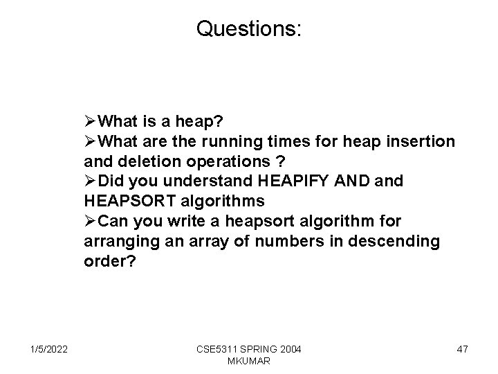
Questions: ØWhat is a heap? ØWhat are the running times for heap insertion and deletion operations ? ØDid you understand HEAPIFY AND and HEAPSORT algorithms ØCan you write a heapsort algorithm for arranging an array of numbers in descending order? 1/5/2022 CSE 5311 SPRING 2004 MKUMAR 47