CMSC 471 Fall 2002 Class 27 28 Monday

CMSC 471 Fall 2002 Class #27 -28 – Monday, December 2 / Wednesday, December 4 1

Today’s class(es) • Neural networks • Bayesian learning 2

Neural Networks / Bayes Net Learning Chapter 19 Some material adapted from lecture notes by Lise Getoor and Ron Parr 3

Neural function • Brain function (thought) occurs as the result of the firing of neurons • Neurons connect to each other through synapses, which propagate action potential (electrical impulses) by releasing neurotransmitters • Synapses can be excitatory (potential-increasing) or inhibitory (potential-decreasing), and have varying activation thresholds • Learning occurs as a result of the synapses’ plasticicity: They exhibit long-term changes in connection strength • There about 1011 neurons and about 1014 synapses in the human brain(!) 4

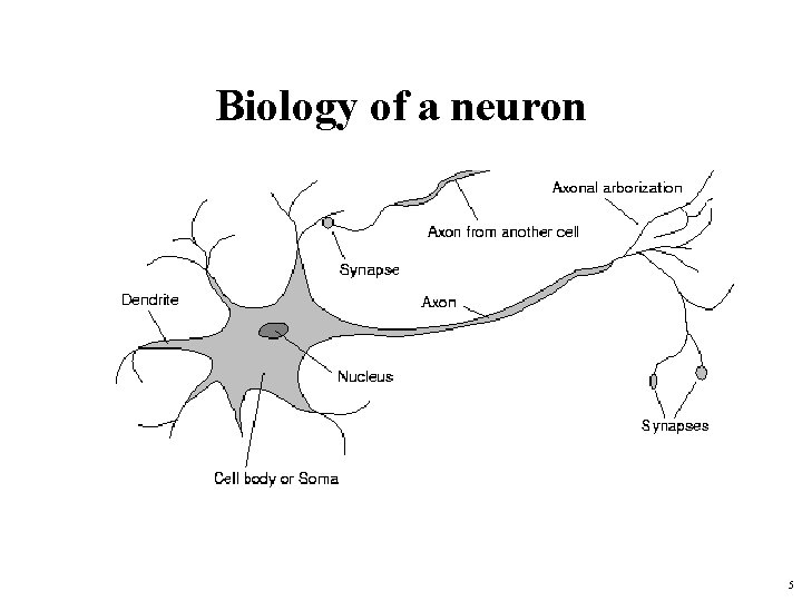
Biology of a neuron 5

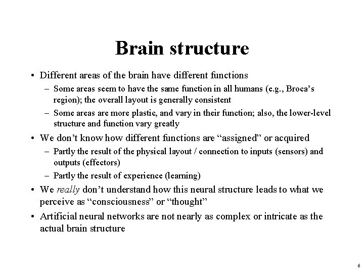
Brain structure • Different areas of the brain have different functions – Some areas seem to have the same function in all humans (e. g. , Broca’s region); the overall layout is generally consistent – Some areas are more plastic, and vary in their function; also, the lower-level structure and function vary greatly • We don’t know how different functions are “assigned” or acquired – Partly the result of the physical layout / connection to inputs (sensors) and outputs (effectors) – Partly the result of experience (learning) • We really don’t understand how this neural structure leads to what we perceive as “consciousness” or “thought” • Artificial neural networks are not nearly as complex or intricate as the actual brain structure 6

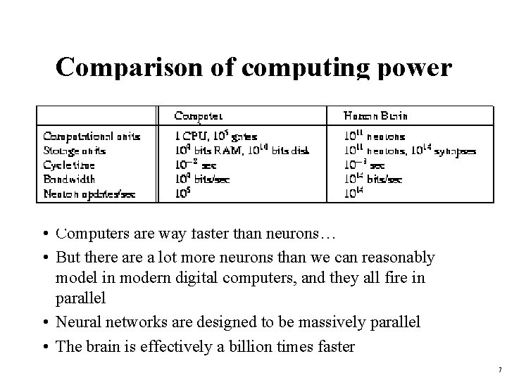
Comparison of computing power • Computers are way faster than neurons… • But there a lot more neurons than we can reasonably model in modern digital computers, and they all fire in parallel • Neural networks are designed to be massively parallel • The brain is effectively a billion times faster 7

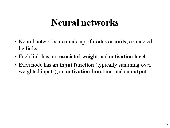
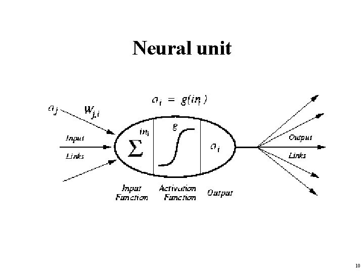
Neural networks • Neural networks are made up of nodes or units, connected by links • Each link has an associated weight and activation level • Each node has an input function (typically summing over weighted inputs), an activation function, and an output 8

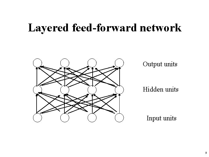
Layered feed-forward network Output units Hidden units Input units 9

Neural unit 10

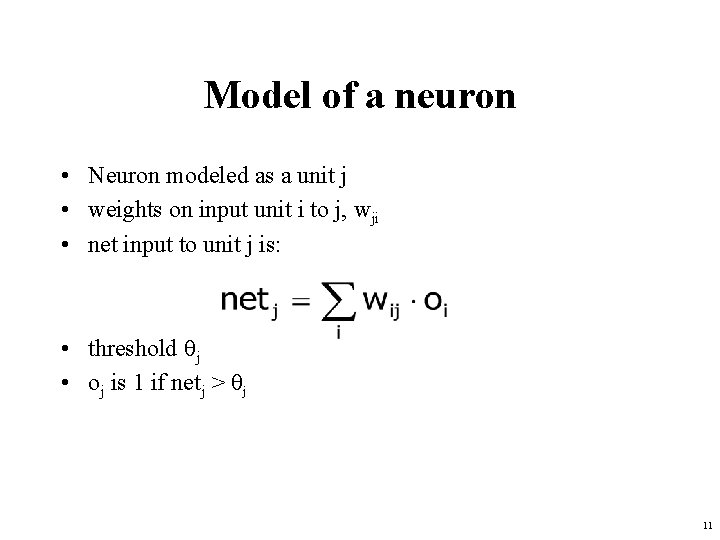
Model of a neuron • Neuron modeled as a unit j • weights on input unit i to j, wji • net input to unit j is: • threshold j • oj is 1 if netj > j 11

“Executing” neural networks • Input units are set by some exterior function (think of these as sensors), which causes their output links to be activated at the specified level • Working forward through the network, the input function of each unit is applied to compute the input value – Usually this is just the weighted sum of the activation on the links feeding into this node • The activation function transforms this input function into a final value – Typically this is a nonlinear function, often a sigmoid function corresponding to the “threshold” of that node 12

Learning rules • Rosenblatt (1959) suggested that if a target output value is provided for a single neuron with fixed inputs, can incrementally change weights to learn to produce these outputs using the perceptron learning rule – assumes binary valued input/outputs – assumes a single linear threshold unit 13

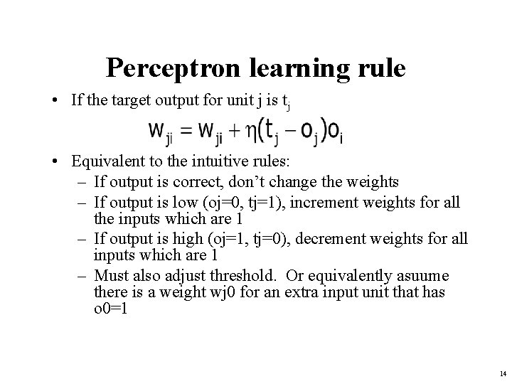
Perceptron learning rule • If the target output for unit j is tj • Equivalent to the intuitive rules: – If output is correct, don’t change the weights – If output is low (oj=0, tj=1), increment weights for all the inputs which are 1 – If output is high (oj=1, tj=0), decrement weights for all inputs which are 1 – Must also adjust threshold. Or equivalently asuume there is a weight wj 0 for an extra input unit that has o 0=1 14

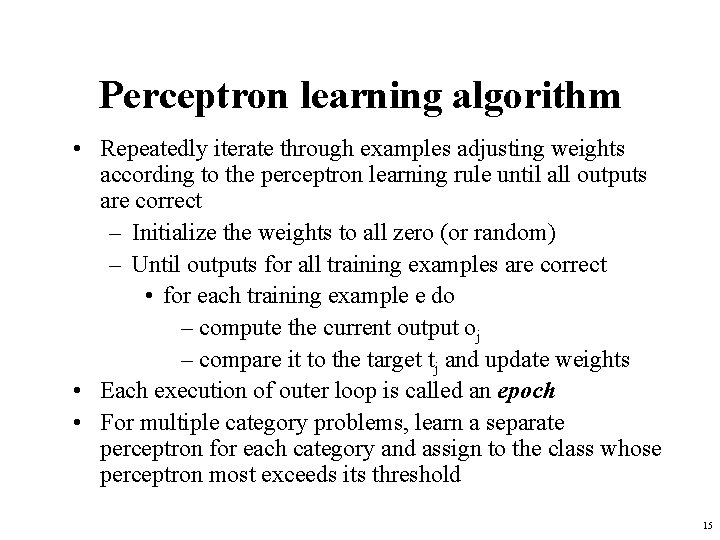
Perceptron learning algorithm • Repeatedly iterate through examples adjusting weights according to the perceptron learning rule until all outputs are correct – Initialize the weights to all zero (or random) – Until outputs for all training examples are correct • for each training example e do – compute the current output oj – compare it to the target tj and update weights • Each execution of outer loop is called an epoch • For multiple category problems, learn a separate perceptron for each category and assign to the class whose perceptron most exceeds its threshold 15

Representation limitations of a perceptron • Perceptrons can only represent linear threshold functions and can therefore only learn functions which linearly separate the data: i. e. , the positive and negative examples are separable by a hyperplane in n-dimensional space 16

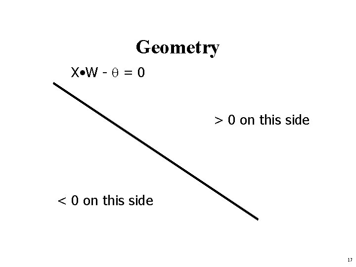
Geometry X • W - = 0 > 0 on this side < 0 on this side 17

Perceptron learnability • Perceptron Convergence Theorem: If there is a set of weights that is consistent with the training data (i. e. , the data is linearly separable), the perceptron learning algorithm will converge (Minicksy & Papert, 1969) • Unfortunately, many functions (like parity) cannot be represented by LTU 18

Learning: Backpropagation • Similar to perceptron learning algorithm, we cycle through our examples – if the output of the network is correct, no changes are made – if there is an error, the weights are adjusted to reduce the error • The trick is to assess the blame for the error and divide it among the contributing weights 19

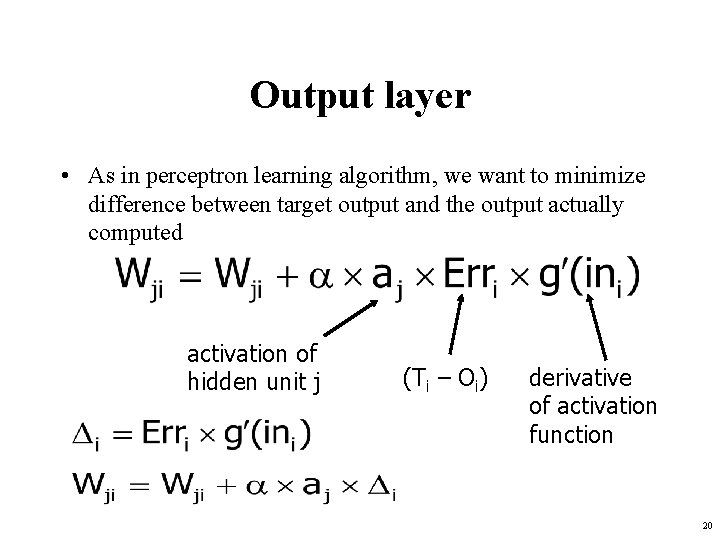
Output layer • As in perceptron learning algorithm, we want to minimize difference between target output and the output actually computed activation of hidden unit j (Ti – Oi) derivative of activation function 20

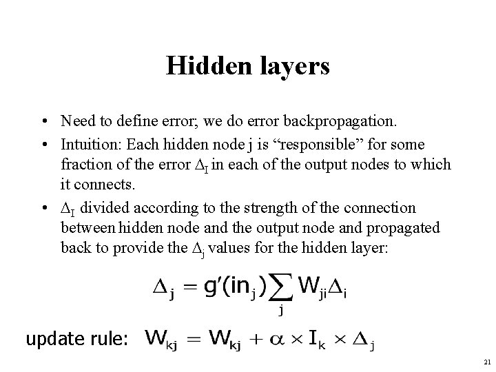
Hidden layers • Need to define error; we do error backpropagation. • Intuition: Each hidden node j is “responsible” for some fraction of the error I in each of the output nodes to which it connects. • I divided according to the strength of the connection between hidden node and the output node and propagated back to provide the j values for the hidden layer: update rule: 21

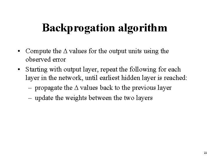
Backprogation algorithm • Compute the values for the output units using the observed error • Starting with output layer, repeat the following for each layer in the network, until earliest hidden layer is reached: – propagate the values back to the previous layer – update the weights between the two layers 22

Backprop issues • “Backprop is the cockroach of machine learning. It’s ugly, and annoying, but you just can’t get rid of it. ” Geoff Hinton • Problems: – black box – local minima 23

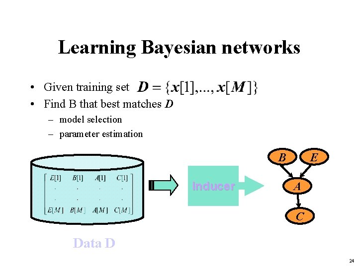
Learning Bayesian networks • Given training set • Find B that best matches D – model selection – parameter estimation B Inducer E A C Data D 24

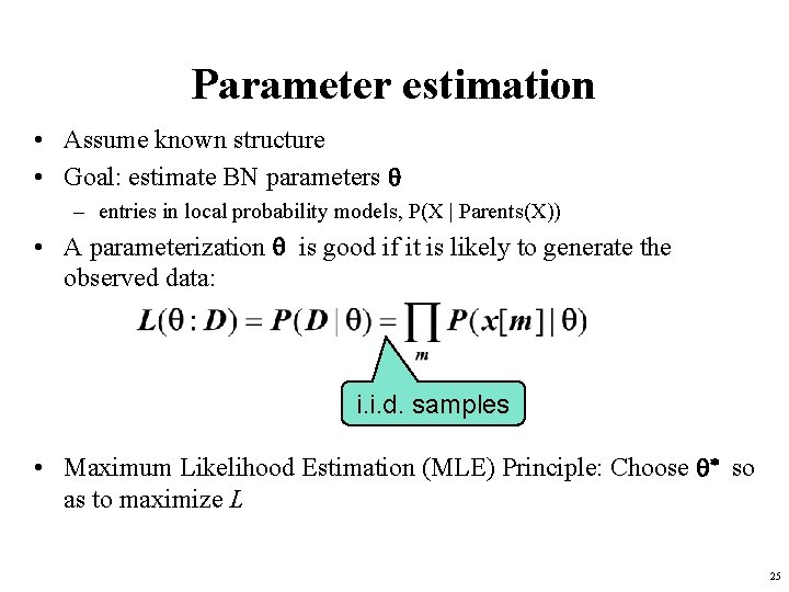
Parameter estimation • Assume known structure • Goal: estimate BN parameters q – entries in local probability models, P(X | Parents(X)) • A parameterization q is good if it is likely to generate the observed data: i. i. d. samples • Maximum Likelihood Estimation (MLE) Principle: Choose q* so as to maximize L 25

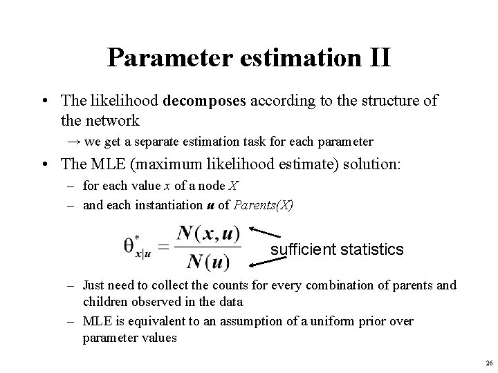
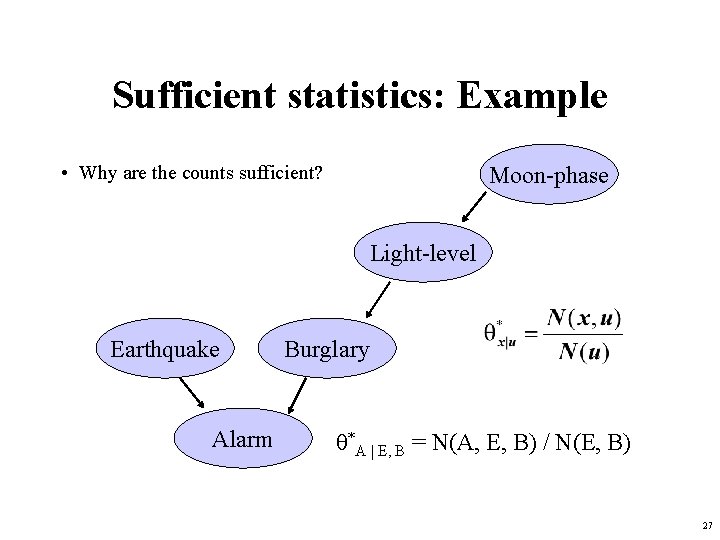
Parameter estimation II • The likelihood decomposes according to the structure of the network → we get a separate estimation task for each parameter • The MLE (maximum likelihood estimate) solution: – for each value x of a node X – and each instantiation u of Parents(X) sufficient statistics – Just need to collect the counts for every combination of parents and children observed in the data – MLE is equivalent to an assumption of a uniform prior over parameter values 26

Sufficient statistics: Example • Why are the counts sufficient? Moon-phase Light-level Earthquake Alarm Burglary θ*A | E, B = N(A, E, B) / N(E, B) 27

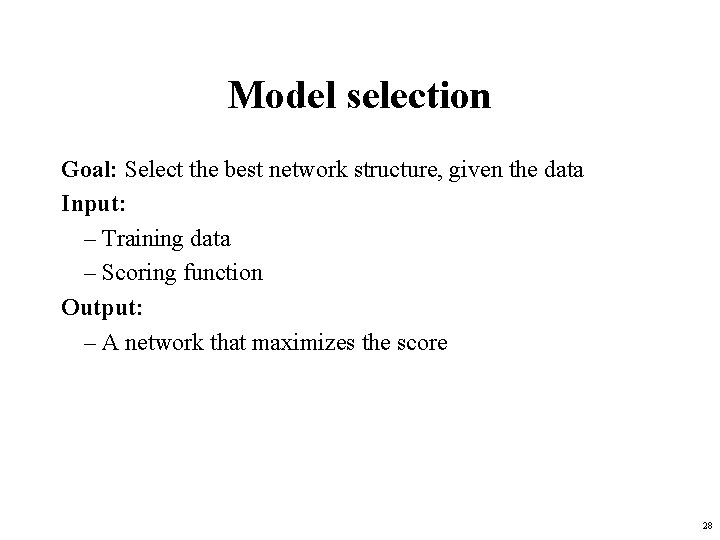
Model selection Goal: Select the best network structure, given the data Input: – Training data – Scoring function Output: – A network that maximizes the score 28

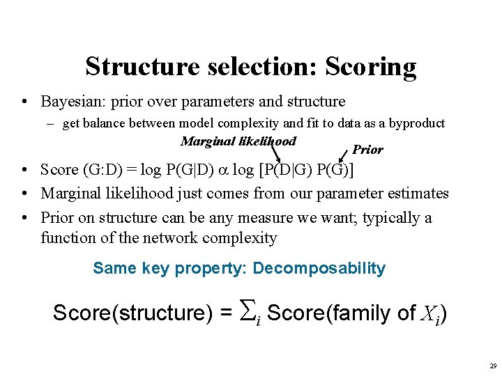
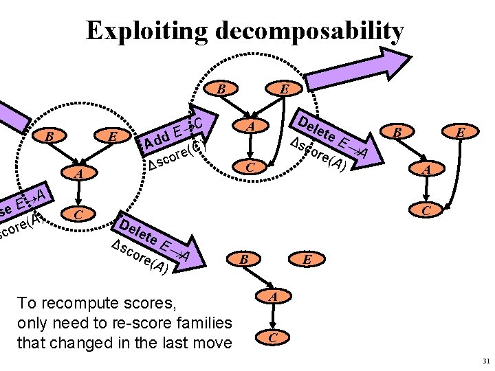
Structure selection: Scoring • Bayesian: prior over parameters and structure – get balance between model complexity and fit to data as a byproduct Marginal likelihood Prior • Score (G: D) = log P(G|D) log [P(D|G) P(G)] • Marginal likelihood just comes from our parameter estimates • Prior on structure can be any measure we want; typically a function of the network complexity Same key property: Decomposability Score(structure) = Si Score(family of Xi) 29

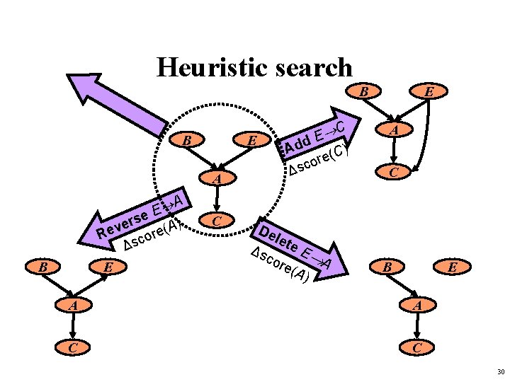
Heuristic search B B E A A E se r ) e A v ( e e R or c s Δ E B C C E Add (C) re o c Δs De let e. E Δs A cor e(A ) E A C B E A A C C 30

Exploiting decomposability B B E A A E se ) A ( e r sco C C E Add (C) re o c Δs De let e. E Δs A cor e(A ) To recompute scores, only need to re-score families that changed in the last move E De let e. E Δs A cor e(A ) A C B E A C 31