Class 23 The most overrated statistic The four

Class 23 The most over-rated statistic The four assumptions The most Important hypothesis test yet Using yes/no variables in regressions

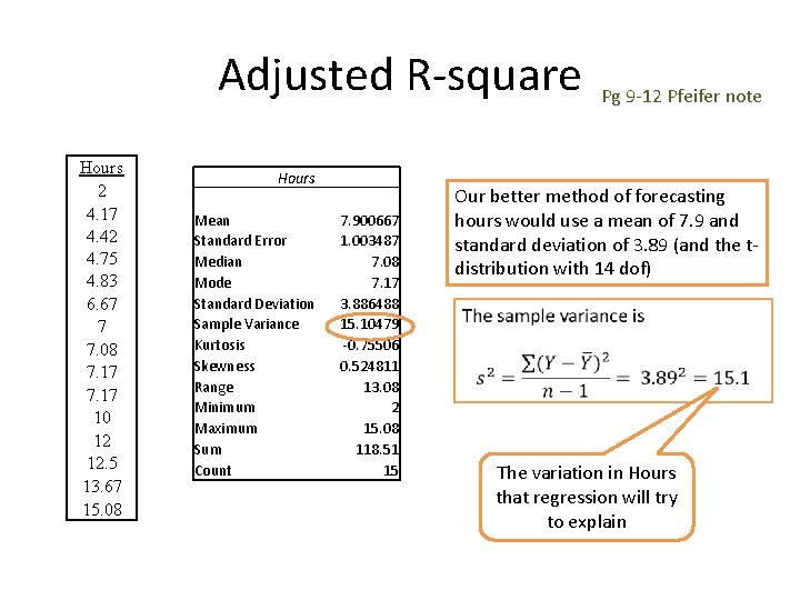
Adjusted R-square Hours 2 4. 17 4. 42 4. 75 4. 83 6. 67 7 7. 08 7. 17 10 12 12. 5 13. 67 15. 08 Hours Mean 7. 900667 Standard Error 1. 003487 Median 7. 08 Mode 7. 17 Standard Deviation 3. 886488 Sample Variance 15. 10479 Kurtosis -0. 75506 Skewness 0. 524811 Range 13. 08 Minimum 2 Maximum 15. 08 Sum 118. 51 Count 15 Pg 9 -12 Pfeifer note Our better method of forecasting hours would use a mean of 7. 9 and standard deviation of 3. 89 (and the tdistribution with 14 dof) The variation in Hours that regression will try to explain

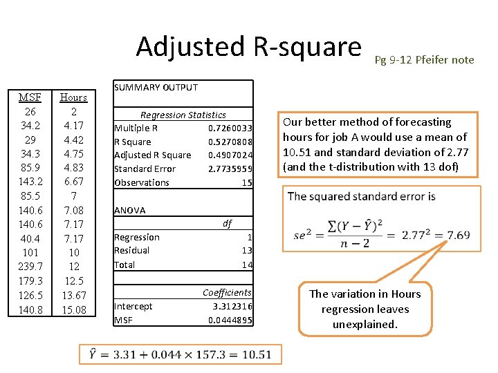
Adjusted R-square MSF 26 34. 2 29 34. 3 85. 9 143. 2 85. 5 140. 6 40. 4 101 239. 7 179. 3 126. 5 140. 8 Hours 2 4. 17 4. 42 4. 75 4. 83 6. 67 7 7. 08 7. 17 10 12 12. 5 13. 67 15. 08 SUMMARY OUTPUT Regression Statistics Multiple R 0. 7260033 R Square 0. 5270808 Adjusted R Square 0. 4907024 Standard Error 2. 7735959 Observations 15 ANOVA df Regression 1 Residual 13 Total 14 Coefficients Intercept 3. 312316 MSF 0. 0444895 Pg 9 -12 Pfeifer note Our better method of forecasting hours for job A would use a mean of 10. 51 and standard deviation of 2. 77 (and the t-distribution with 13 dof) The variation in Hours regression leaves unexplained.

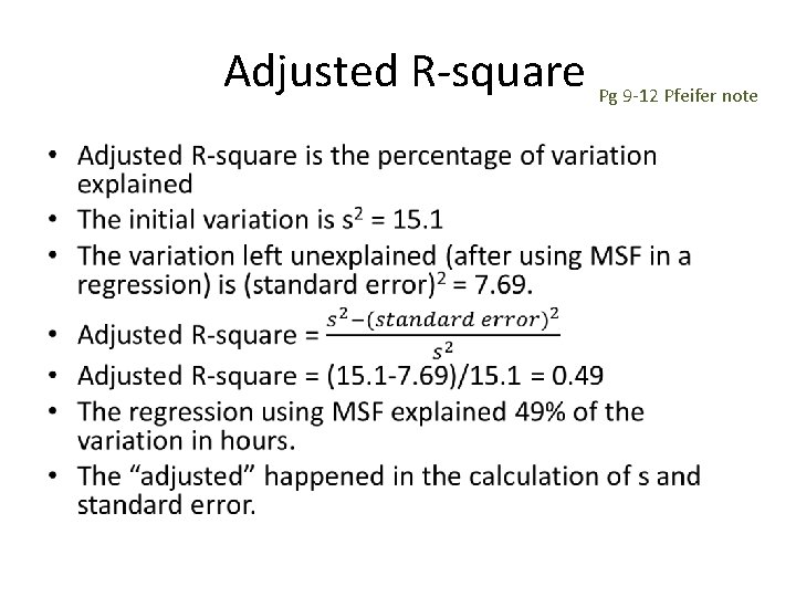
Adjusted R-square Pg 9 -12 Pfeifer note •

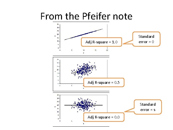
From the Pfeifer note Adj R-square = 1. 0 Standard error = 0 Adj R-square = 0. 5 Standard error = s Adj R-square = 0. 0

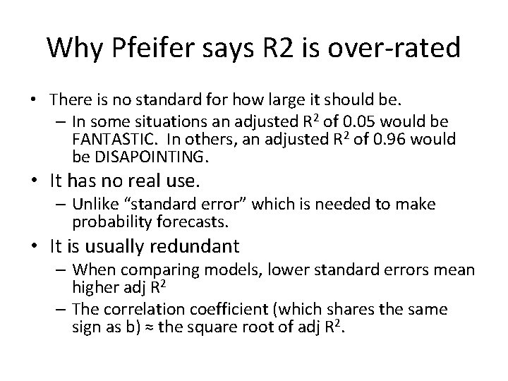
Why Pfeifer says R 2 is over-rated • There is no standard for how large it should be. – In some situations an adjusted R 2 of 0. 05 would be FANTASTIC. In others, an adjusted R 2 of 0. 96 would be DISAPOINTING. • It has no real use. – Unlike “standard error” which is needed to make probability forecasts. • It is usually redundant – When comparing models, lower standard errors mean higher adj R 2 – The correlation coefficient (which shares the same sign as b) ≈ the square root of adj R 2.

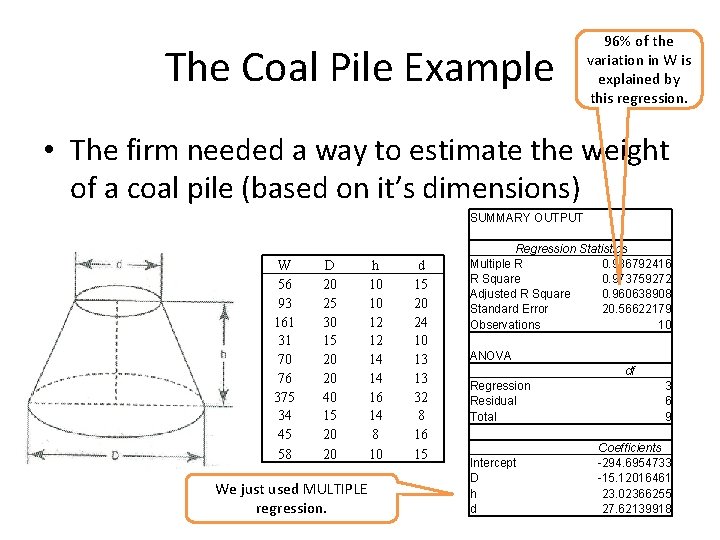
The Coal Pile Example 96% of the variation in W is explained by this regression. • The firm needed a way to estimate the weight of a coal pile (based on it’s dimensions) W 56 93 161 31 70 76 375 34 45 58 D 20 25 30 15 20 20 40 15 20 20 h 10 10 12 12 14 14 16 14 8 10 We just used MULTIPLE regression. d 15 20 24 10 13 13 32 8 16 15 SUMMARY OUTPUT Regression Statistics Multiple R 0. 986792416 R Square 0. 973759272 Adjusted R Square 0. 960638908 Standard Error 20. 56622179 Observations 10 ANOVA df Regression 3 Residual 6 Total 9 Coefficients Intercept -294. 6954733 D -15. 12016461 h 23. 02366255 d 27. 62139918

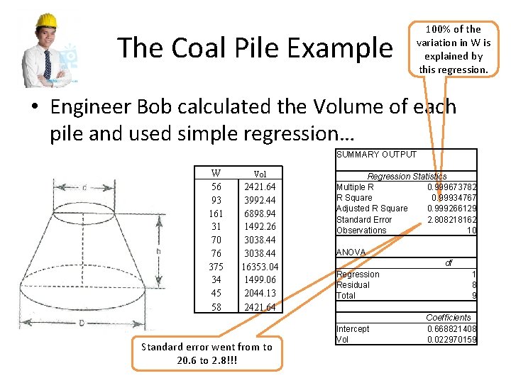
The Coal Pile Example 100% of the variation in W is explained by this regression. • Engineer Bob calculated the Volume of each pile and used simple regression… W 56 93 161 31 70 76 375 34 45 58 Vol 2421. 64 3992. 44 6898. 94 1492. 26 3038. 44 16353. 04 1499. 06 2044. 13 2421. 64 Standard error went from to 20. 6 to 2. 8!!! SUMMARY OUTPUT Regression Statistics Multiple R 0. 999673782 R Square 0. 99934767 Adjusted R Square 0. 999266129 Standard Error 2. 808218162 Observations 10 ANOVA df Regression 1 Residual 8 Total 9 Coefficients Intercept 0. 668821408 Vol 0. 022970159

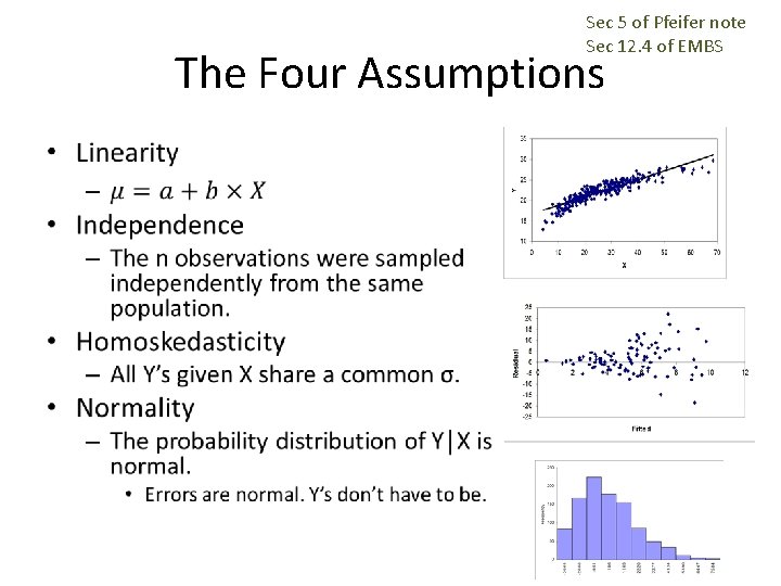
Sec 5 of Pfeifer note Sec 12. 4 of EMBS The Four Assumptions •

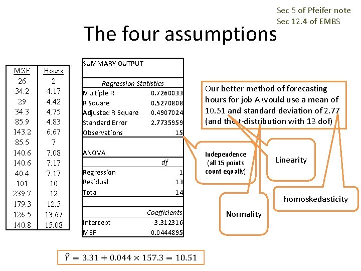
Sec 5 of Pfeifer note Sec 12. 4 of EMBS The four assumptions MSF 26 34. 2 29 34. 3 85. 9 143. 2 85. 5 140. 6 40. 4 101 239. 7 179. 3 126. 5 140. 8 Hours 2 4. 17 4. 42 4. 75 4. 83 6. 67 7 7. 08 7. 17 10 12 12. 5 13. 67 15. 08 SUMMARY OUTPUT Regression Statistics Multiple R 0. 7260033 R Square 0. 5270808 Adjusted R Square 0. 4907024 Standard Error 2. 7735959 Observations 15 ANOVA df Regression 1 Residual 13 Total 14 Coefficients Intercept 3. 312316 MSF 0. 0444895 Our better method of forecasting hours for job A would use a mean of 10. 51 and standard deviation of 2. 77 (and the t-distribution with 13 dof) Independence (all 15 points count equally) Linearity homoskedasticity Normality

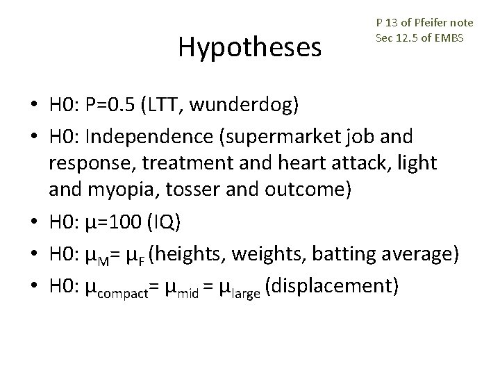
Hypotheses P 13 of Pfeifer note Sec 12. 5 of EMBS • H 0: P=0. 5 (LTT, wunderdog) • H 0: Independence (supermarket job and response, treatment and heart attack, light and myopia, tosser and outcome) • H 0: μ=100 (IQ) • H 0: μM= μF (heights, weights, batting average) • H 0: μcompact= μmid = μlarge (displacement)

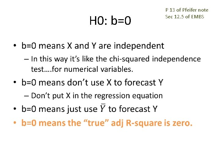
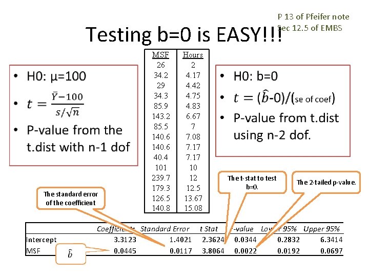
H 0: b=0 • P 13 of Pfeifer note Sec 12. 5 of EMBS

P 13 of Pfeifer note Sec 12. 5 of EMBS Testing b=0 is EASY!!! • The standard error of the coefficient Intercept MSF 26 34. 2 29 34. 3 85. 9 143. 2 85. 5 140. 6 40. 4 101 239. 7 179. 3 126. 5 140. 8 Hours 2 4. 17 4. 42 4. 75 4. 83 6. 67 7 7. 08 7. 17 10 12 12. 5 13. 67 15. 08 • The t-stat to test b=0. The 2 -tailed p-value. Coefficients Standard Error t Stat P-value Lower 95% Upper 95% 3. 3123 1. 4021 2. 3624 0. 0344 0. 2832 6. 3414 0. 0445 0. 0117 3. 8064 0. 0022 0. 0192 0. 0697

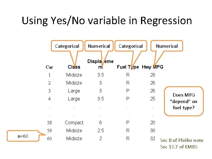
Using Yes/No variable in Regression Categorical n=60 Numerical Categorical Displaceme nt Fuel Type Hwy MPG Car Class 1 Midsize 3. 5 R 28 2 Midsize 3 R 26 3 Large 3 P 26 4 Large 3. 5 P 25 . . 58 Compact 6 P 20 59 Midsize 2. 5 R 30 60 Midsize 2 R 32 Does MPG “depend” on fuel type? Sec 8 of Pfeifer note Sec 13. 7 of EMBS

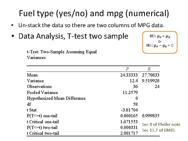
Fuel type (yes/no) and mpg (numerical) • Un-stack the data so there are two columns of MPG data. • Data Analysis, T-test two sample H 0: μP = μR Or H 0: μP – μR = 0 t-Test: Two-Sample Assuming Equal Variances Mean Variance Observations Pooled Variance Hypothesized Mean Difference df t Stat P(T<=t) one-tail t Critical one-tail P(T<=t) two-tail t Critical two-tail P 24. 33333 12. 4 36 11. 2579 0 58 -3. 81704 0. 000165 1. 671553 0. 000331 2. 001717 R 27. 70833 9. 519928 24 0. 999835 Sec 8 of Pfeifer note Sec 13. 7 of EMBS

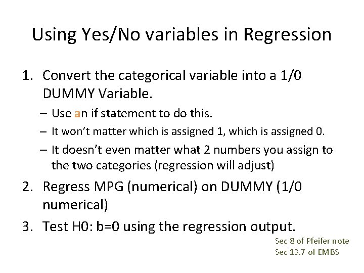
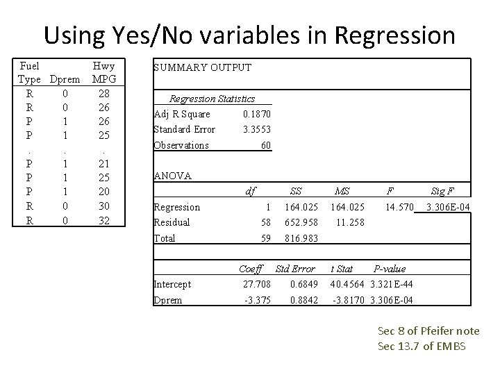
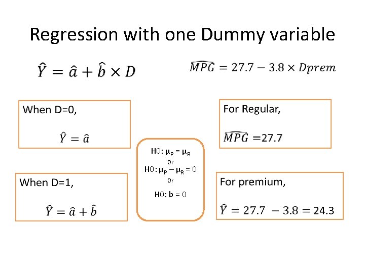
Using Yes/No variables in Regression 1. Convert the categorical variable into a 1/0 DUMMY Variable. – Use an if statement to do this. – It won’t matter which is assigned 1, which is assigned 0. – It doesn’t even matter what 2 numbers you assign to the two categories (regression will adjust) 2. Regress MPG (numerical) on DUMMY (1/0 numerical) 3. Test H 0: b=0 using the regression output. Sec 8 of Pfeifer note Sec 13. 7 of EMBS

Using Yes/No variables in Regression Fuel Type Dprem R 0 P 1. . P 1 P 1 R 0 Hwy MPG 28 26 26 25. 21 25 20 30 32 SUMMARY OUTPUT Regression Statistics Adj R Square 0. 1870 Standard Error 3. 3553 Observations ANOVA df SS 1 58 164. 025 652. 958 Total 59 816. 983 Dprem 60 Regression Residual Intercept MS F 164. 025 11. 258 Sig F 14. 570 3. 306 E-04 Coeff Std Error 27. 708 0. 6849 -3. 375 0. 8842 t Stat P-value 40. 4564 3. 321 E-44 -3. 8170 3. 306 E-04 Sec 8 of Pfeifer note Sec 13. 7 of EMBS

Regression with one Dummy variable H 0: μP = μR Or H 0: μP – μR = 0 Or H 0: b = 0

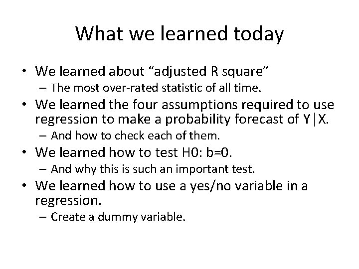
What we learned today • We learned about “adjusted R square” – The most over-rated statistic of all time. • We learned the four assumptions required to use regression to make a probability forecast of Y│X. – And how to check each of them. • We learned how to test H 0: b=0. – And why this is such an important test. • We learned how to use a yes/no variable in a regression. – Create a dummy variable.