Chapter 25 AllPairs Shortest Paths Application Computing distance

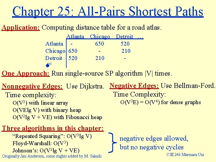
Chapter 25: All-Pairs Shortest Paths Application: Computing distance table for a road atlas. Atlanta Chicago 650 Detroit 520 Chicago 650 210 Detroit … 520 210 - One Approach: Run single-source SP algorithm |V| times. Nonnegative Edges: Use Dijkstra. Negative Edges: Use Bellman-Ford. Time Complexity: Time complexity: O(V 3) with linear array O(VElg V) with binary heap O(V 2 lg V + VE) with Fibonacci heap O(V 2 E) = O(V 4) for dense graphs Three algorithms in this chapter: “Repeated Squaring”: O(V 3 lg V) Floyd-Warshall: O(V 3) Johnson’s: O(V 2 lg V + VE) Originally Jim Anderson, some slights added by M. Sakalli negative edges allowed, but no negative cycles CSE 246 Marmara Uni

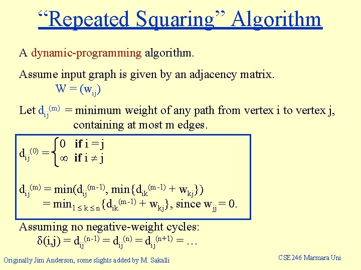
“Repeated Squaring” Algorithm A dynamic-programming algorithm. Assume input graph is given by an adjacency matrix. W = (wij) Let dij(m) = minimum weight of any path from vertex i to vertex j, containing at most m edges. dij (0) 0 if i = j = if i j dij(m) = min(dij(m-1), min{dik(m-1) + wkj}) = min 1 k n{dik(m-1) + wkj}, since wjj = 0. Assuming no negative-weight cycles: δ(i, j) = dij(n-1) = dij(n+1) = … Originally Jim Anderson, some slights added by M. Sakalli CSE 246 Marmara Uni

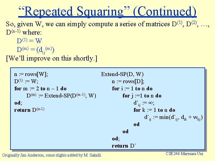
“Repeated Squaring” (Continued) So, given W, we can simply compute a series of matrices D(1), D(2), …, D(n-1) where: D(1) = W D(m) = (dij(m)) [We’ll improve on this shortly. ] Extend-SP(D, W) n : = rows[W]; n : = rows[D]; D(1) : = W; for i : = 1 to n do for m : = 2 to n – 1 do for j : =1 to n do D(m) : = Extend-SP(D(m-1), W) d´ij : = ; od; for k : = 1 to n do return D(n-1) d´ij : = min(d´ij, dik + wkj) od od od; return D´ Originally Jim Anderson, some slights added by M. Sakalli CSE 246 Marmara Uni

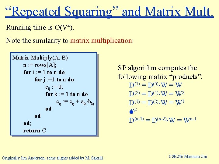
“Repeated Squaring” and Matrix Mult. Running time is O(V 4). Note the similarity to matrix multiplication: Matrix-Multiply(A, B) n : = rows[A]; for i : = 1 to n do for j : =1 to n do cij : = 0; for k : = 1 to n do cij : = cij + aik bkj od od od; return C Originally Jim Anderson, some slights added by M. Sakalli SP algorithm computes the following matrix “products”: D(1) = D(0) W = W D(2) = D(1) W = W 2 D(3) = D(2) W = W 3 D(n-1) = D(n-2) W = Wn-1 CSE 246 Marmara Uni

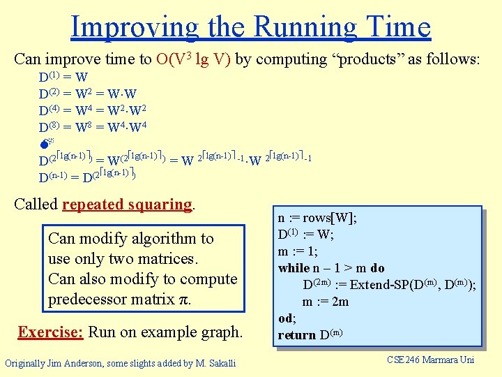
Improving the Running Time Can improve time to O(V 3 lg V) by computing “products” as follows: D(1) = W D(2) = W 2 = W W D(4) = W 4 = W 2 D(8) = W 8 = W 4 lg(n-1) ) lg(n-1) -1 D(2 = W(2 =W 2 lg(n-1) ) D(n-1) = D(2 Called repeated squaring. Can modify algorithm to use only two matrices. Can also modify to compute predecessor matrix π. Exercise: Run on example graph. Originally Jim Anderson, some slights added by M. Sakalli n : = rows[W]; D(1) : = W; m : = 1; while n – 1 > m do D(2 m) : = Extend-SP(D(m), D(m)); m : = 2 m od; return D(m) CSE 246 Marmara Uni

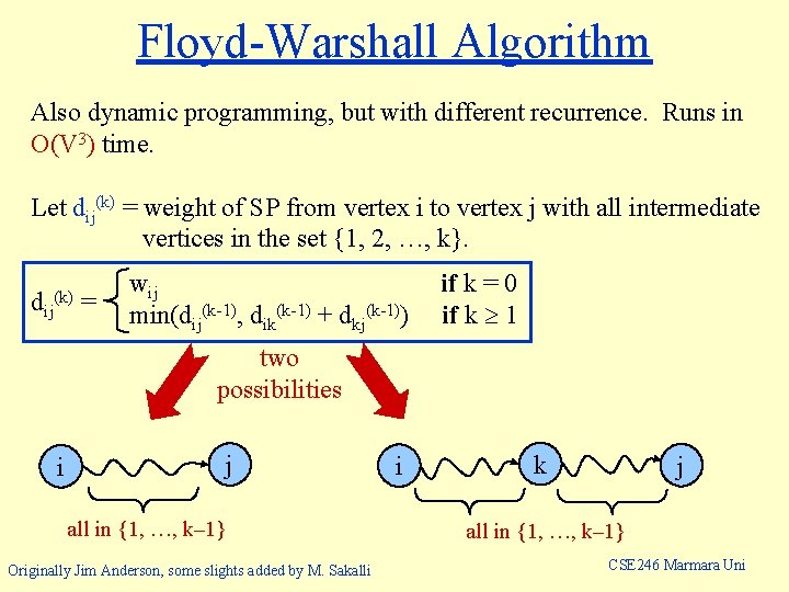
Floyd-Warshall Algorithm Also dynamic programming, but with different recurrence. Runs in O(V 3) time. Let dij(k) = weight of SP from vertex i to vertex j with all intermediate vertices in the set {1, 2, …, k}. dij (k) = wij min(dij(k-1), dik(k-1) + dkj(k-1)) if k = 0 if k 1 two possibilities j i all in {1, …, k– 1} Originally Jim Anderson, some slights added by M. Sakalli i k j all in {1, …, k– 1} CSE 246 Marmara Uni

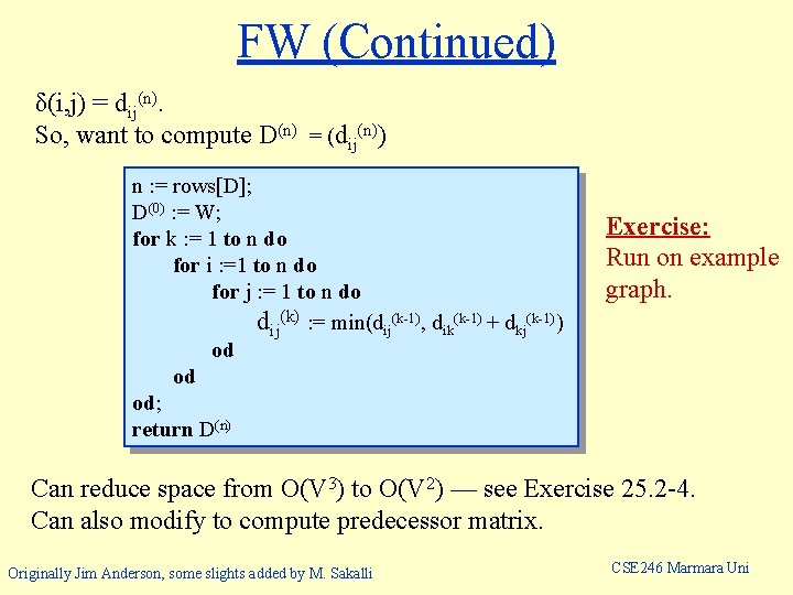
FW (Continued) δ(i, j) = dij(n). So, want to compute D(n) = (dij(n)) n : = rows[D]; D(0) : = W; for k : = 1 to n do for i : =1 to n do for j : = 1 to n do dij(k) : = min(dij(k-1), dik(k-1) + dkj(k-1)) od od od; return D(n) Exercise: Run on example graph. Can reduce space from O(V 3) to O(V 2) — see Exercise 25. 2 -4. Can also modify to compute predecessor matrix. Originally Jim Anderson, some slights added by M. Sakalli CSE 246 Marmara Uni

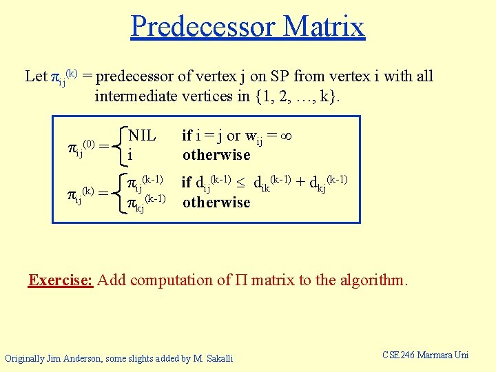
Predecessor Matrix Let πij(k) = predecessor of vertex j on SP from vertex i with all intermediate vertices in {1, 2, …, k}. πij (0) = πij(k) = NIL i if i = j or wij = otherwise πij(k-1) if dij(k-1) dik(k-1) + dkj(k-1) πkj(k-1) otherwise Exercise: Add computation of matrix to the algorithm. Originally Jim Anderson, some slights added by M. Sakalli CSE 246 Marmara Uni

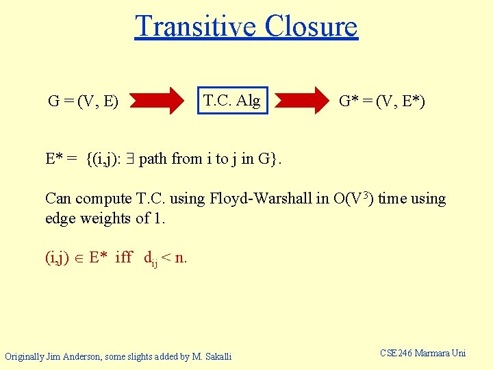
Transitive Closure G = (V, E) T. C. Alg G* = (V, E*) E* = {(i, j): path from i to j in G}. Can compute T. C. using Floyd-Warshall in O(V 3) time using edge weights of 1. (i, j) E* iff dij < n. Originally Jim Anderson, some slights added by M. Sakalli CSE 246 Marmara Uni

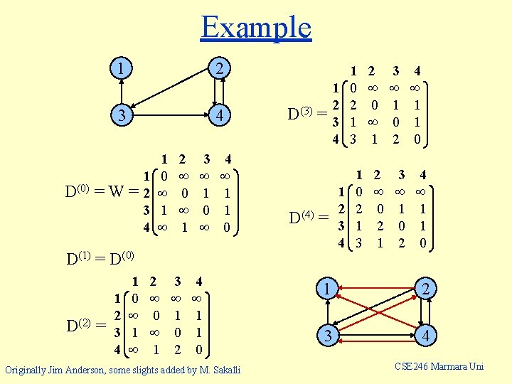
Example 1 2 3 4 D(0) = W = 1 2 3 4 1 0 1 2 3 0 1 4 1 1 0 D(3) = 1 2 3 4 D(4) = D(1) = D(0) D(2) = 1 2 3 4 1 0 1 2 3 0 1 2 4 1 1 0 Originally Jim Anderson, some slights added by M. Sakalli 1 2 3 4 1 0 2 1 3 2 3 0 1 2 4 1 1 0 1 2 3 4 CSE 246 Marmara Uni

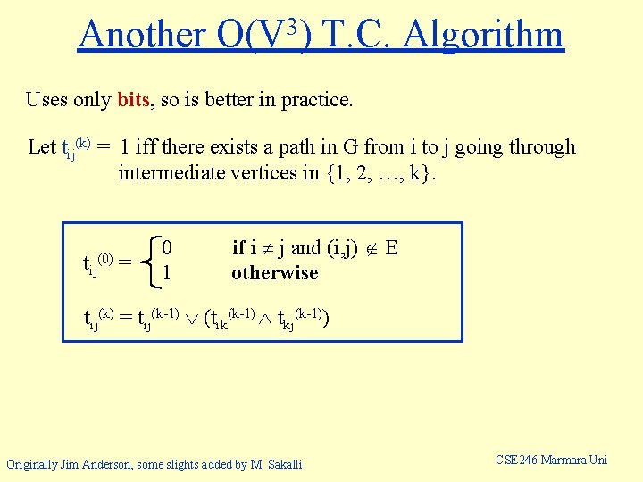
Another 3 O(V ) T. C. Algorithm Uses only bits, so is better in practice. Let tij(k) = 1 iff there exists a path in G from i to j going through intermediate vertices in {1, 2, …, k}. tij (0) = 0 1 if i j and (i, j) E otherwise tij(k) = tij(k-1) (tik(k-1) tkj(k-1)) Originally Jim Anderson, some slights added by M. Sakalli CSE 246 Marmara Uni

Code TC(G) n : = |V[G]|; for i : = 1 to n do for j : =1 to n do od if i = j or (i, j) E then tij(0) : = 1 else tij(0) : = 0 fi od; for k : = 1 to n do for i : =1 to n do for j : = 1 to n do od tij(k) : = tij(k-1) (tik(k-1) tkj(k-1)) od od; return T(n) See book for how this algorithm runs on previous example. Originally Jim Anderson, some slights added by M. Sakalli CSE 246 Marmara Uni

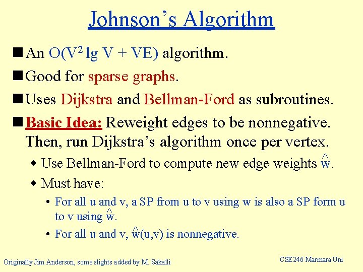
Johnson’s Algorithm n An O(V 2 lg V + VE) algorithm. n Good for sparse graphs. n Uses Dijkstra and Bellman-Ford as subroutines. n Basic Idea: Reweight edges to be nonnegative. Then, run Dijkstra’s algorithm once per vertex. ^ w Use Bellman-Ford to compute new edge weights w. w Must have: • For all u and v, a SP from u to v using w is also a SP form u ^ to v using w. ^ • For all u and v, w(u, v) is nonnegative. Originally Jim Anderson, some slights added by M. Sakalli CSE 246 Marmara Uni

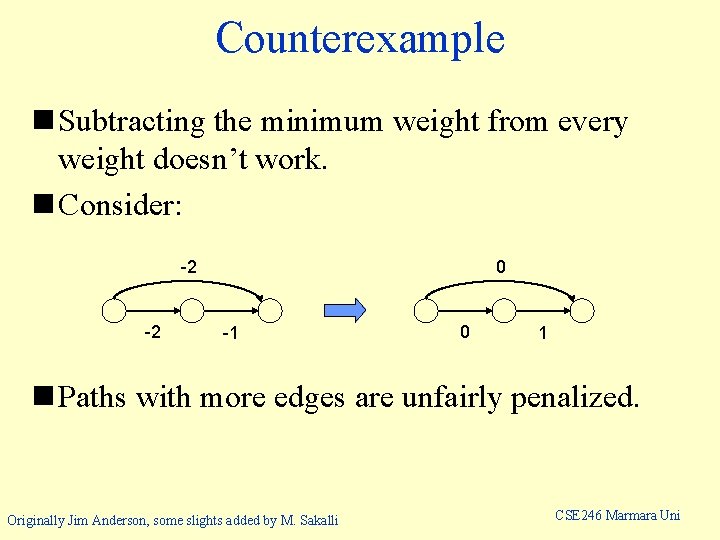
Counterexample n Subtracting the minimum weight from every weight doesn’t work. n Consider: -2 -2 0 -1 0 1 n Paths with more edges are unfairly penalized. Originally Jim Anderson, some slights added by M. Sakalli CSE 246 Marmara Uni

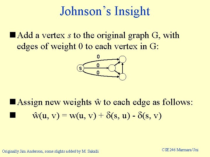
Johnson’s Insight n Add a vertex s to the original graph G, with edges of weight 0 to each vertex in G: 0 s 0 0 n Assign new weights ŵ to each edge as follows: n ŵ(u, v) = w(u, v) + (s, u) - (s, v) Originally Jim Anderson, some slights added by M. Sakalli CSE 246 Marmara Uni

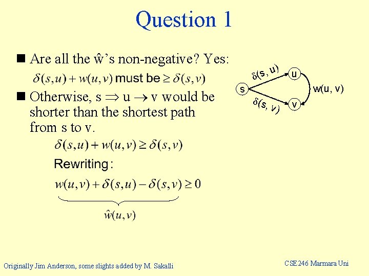
Question 1 n Are all the ŵ’s non-negative? Yes: n Otherwise, s u v would be shorter than the shortest path from s to v. Originally Jim Anderson, some slights added by M. Sakalli ) u , s ( s (s, u w(u, v) v) v CSE 246 Marmara Uni

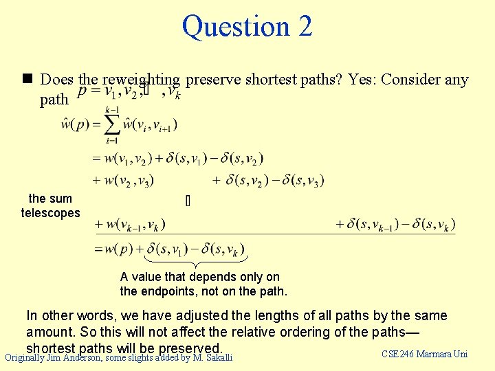
Question 2 n Does the reweighting preserve shortest paths? Yes: Consider any path the sum telescopes A value that depends only on the endpoints, not on the path. In other words, we have adjusted the lengths of all paths by the same amount. So this will not affect the relative ordering of the paths— shortest paths will be preserved. CSE 246 Marmara Uni Originally Jim Anderson, some slights added by M. Sakalli

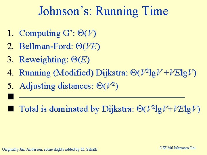
Johnson’s: Running Time 1. 2. 3. 4. 5. n n Computing G’: (V) Bellman-Ford: (VE) Reweighting: (E) Running (Modified) Dijkstra: (V 2 lg. V +VElg. V) Adjusting distances: (V 2) ————————— Total is dominated by Dijkstra: (V 2 lg. V+VElg. V) Originally Jim Anderson, some slights added by M. Sakalli CSE 246 Marmara Uni

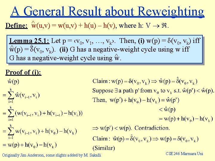
A General Result about Reweighting ^ Define: w(u, v) = w(u, v) + h(u) – h(v), where h: V . Lemma 25. 1: Let p = ‹v 0, v 1, …, vk›. Then, (i) w(p) = δ(v 0, vk) iff ^ w(p) = ^δ(v 0, vk). (ii) G has a negative-weight cycle using w iff ^ G has a negative-weight cycle using w. Proof of (i): Originally Jim Anderson, some slights added by M. Sakalli CSE 246 Marmara Uni

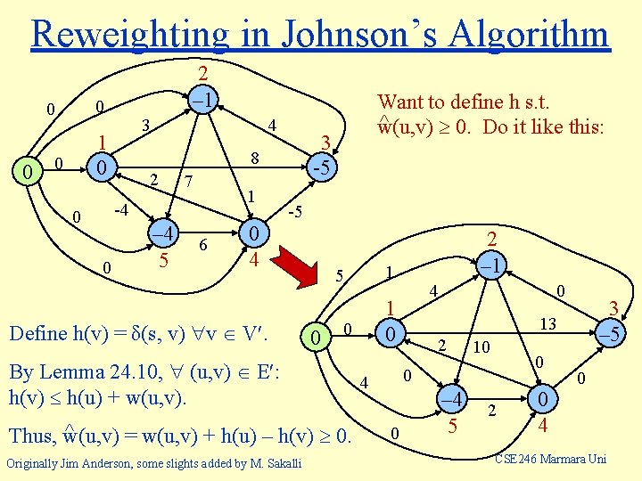
Reweighting in Johnson’s Algorithm 0 0 0 2 – 1 3 1 0 0 4 7 1 -4 0 0 3 -5 8 2 – 4 5 6 Want to define h s. t. ^ w(u, v) 0. Do it like this: -5 0 4 Define h(v) = δ(s, v) v V. ^ Thus, w(u, v) = w(u, v) + h(u) – h(v) 0. 4 1 0 0 By Lemma 24. 10, (u, v) E : h(v) h(u) + w(u, v). Originally Jim Anderson, some slights added by M. Sakalli 1 5 0 2 – 1 0 13 2 10 0 0 4 0 3 – 5 – 4 5 2 0 0 4 CSE 246 Marmara Uni

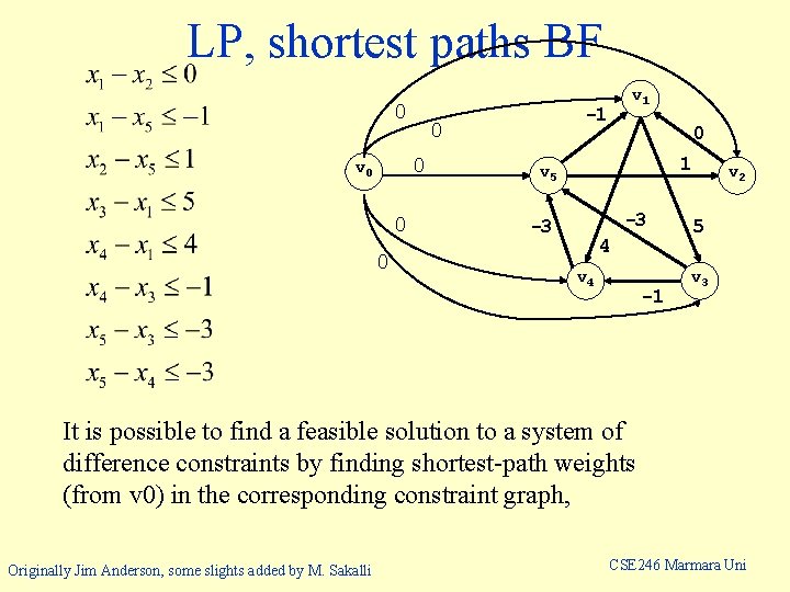
LP, shortest paths BF 0 0 0 -1 0 0 v 1 0 1 v 5 -3 -3 4 v 4 -1 v 2 5 v 3 It is possible to find a feasible solution to a system of difference constraints by finding shortest-path weights (from v 0) in the corresponding constraint graph, Originally Jim Anderson, some slights added by M. Sakalli CSE 246 Marmara Uni

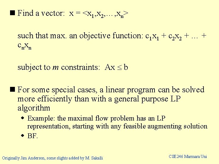
n Find a vector: x = <x 1, x 2, …, xn> such that max. an objective function: c 1 x 1 + c 2 x 2 + … + cnxn subject to m constraints: Ax b n For some special cases, a linear program can be solved more efficiently than with a general purpose LP algorithm w Example: the maximal flow problem has an LP representation, starting with any feasible augmenting solution w BF. Originally Jim Anderson, some slights added by M. Sakalli CSE 246 Marmara Uni

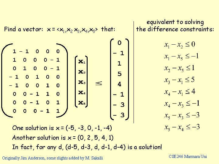
Find a vector: x = <x 1, x 2 x 3, x 4, x 5> that: equivalent to solving the difference constraints: One solution is x = (-5, -3, 0, -1, -4) Another solution is x = (0, 2, 5, 4, 1) In fact, for any d, (d-5, d-3, d, d-1, d-4) is a solution! Originally Jim Anderson, some slights added by M. Sakalli CSE 246 Marmara Uni

Code for Johnson’s Algorithm Compute G´, where V[G´] = V[G] {s}, E[G´] = E[G] {(s, v): v V[G]}; if Bellman-Ford(G´, w, s) = false then negative-weight cycle else for each v V[G´] do set h(v) to (s, v) computed by Bellman-Ford od; Running time for each (u, v) E[G´] do ^ is O(V 2 lg V + VE). w(u, v) : = w(u, v) + h(u) – h(v) od; See Book. for each u V[G] do ^ v) for all v V[G]; ^ u) to compute (u, run Dijkstra(G, w, for each v V[G] do ^ v) + h(v) – h(u) duv : = (u, od od fi Originally Jim Anderson, some slights added by M. Sakalli CSE 246 Marmara Uni

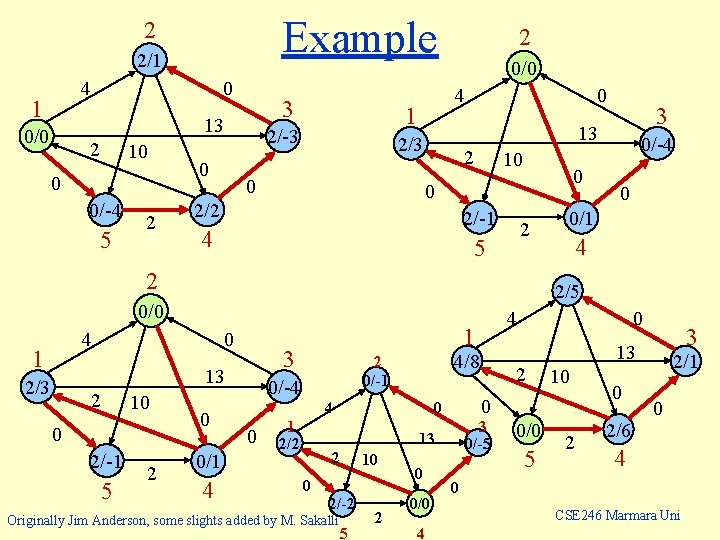
Example 2 2/1 4 1 0 3 13 0/0 2 10 0 0/-4 5 2 0 0/0 4 1 2/-3 2 2 10 0 0 2/2 2/-1 4 2 5 2 4 0 2 10 0 2/-1 5 2 0 0/1 4 4 1 2/2 3 0/-5 13 10 0 2/-2 Originally Jim Anderson, some slights added by M. Sakalli 5 2 0 0/0 4 2 10 0 0 2 0 3 13 4/8 2 0/-1 0/-4 0 4 1 3 13 2/3 0/-4 2/5 0/0 1 3 13 2/3 0 0 0/0 5 2 0 2/6 2/1 0 4 0 CSE 246 Marmara Uni