Chapter 14 Spatial autoregressive models 1 He F

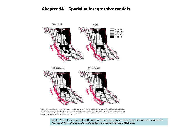
Chapter 14 – Spatial autoregressive models 1 He, F. , Zhou, J. and Zhu, H. T. 2003. Autologistic regression model for the distribution of vegetation. Journal of Agricultural, Biological and Environmental Statistics 8: 205 -222.

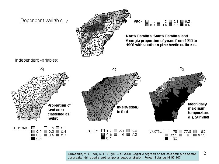
Dependent variable: y North Carolina, South Carolina, and Georgia proportion of years from 1960 to 1990 with southern pine beetle outbreak. Independent variables: x 1 x 2 Proportion of land area classified as hydirc x 3 ln(elevation) in foot Mean daily maximum temperature (F), Summer Gumpertz, M. L. , Wu, C. -T. & Pye, J. M. 2000. Logistic regression for southern pine beetle outbreaks with spatial and temporal autocorrelation. Forest Science 46: 95 -107. 2

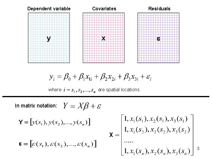
Dependent variable Covariates Residuals y x e where are spatial locations In matrix notation: Y X e 3

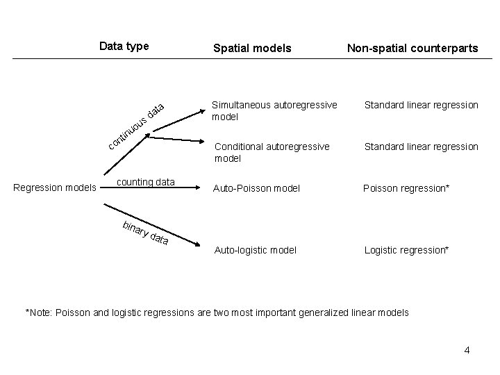
Data type n co Regression models o inu Spatial models a sd ta u t counting data Non-spatial counterparts Simultaneous autoregressive model Standard linear regression Conditional autoregressive model Standard linear regression Auto-Poisson model Poisson regression* Auto-logistic model Logistic regression* bina ry d ata *Note: Poisson and logistic regressions are two most important generalized linear models 4

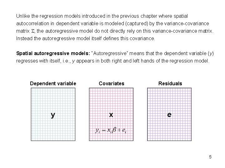
Unlike the regression models introduced in the previous chapter where spatial autocorrelation in dependent variable is modeled (captured) by the variance-covariance matrix , the autoregressive model do not directly rely on this variance-covariance matrix. Instead the autoregressive model itself defines this covariance. Spatial autoregressive models: “Autoregressive” means that the dependent variable (y) regresses with itself, i. e. , y appears in both right and left hands of the regression model. Dependent variable Covariates Residuals y x e 5

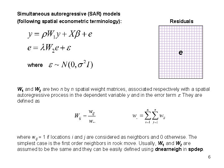
Simultaneous autoregressive (SAR) models (following spatial econometric terminology): Residuals e where W 1 and W 2 are two n by n spatial weight matrices, associated respectively with a spatial autoregressive process in the dependent variable y and in the error term . They are defined as where wij = 1 if locations i and j are considered as neighbors and 0 otherwise. The simplest case is the first order neighbors in rook move. Usually, W 1 and W 2 are assumed to be the same and they can be easily defined using dnearneigh in spdep. 6

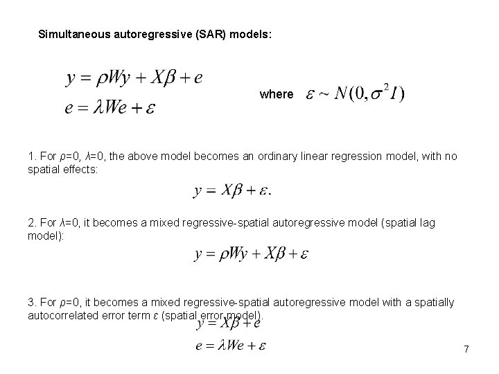
Simultaneous autoregressive (SAR) models: where 1. For ρ=0, λ=0, the above model becomes an ordinary linear regression model, with no spatial effects: 2. For λ=0, it becomes a mixed regressive-spatial autoregressive model (spatial lag model): 3. For ρ=0, it becomes a mixed regressive-spatial autoregressive model with a spatially autocorrelated error term ε (spatial error model). 7

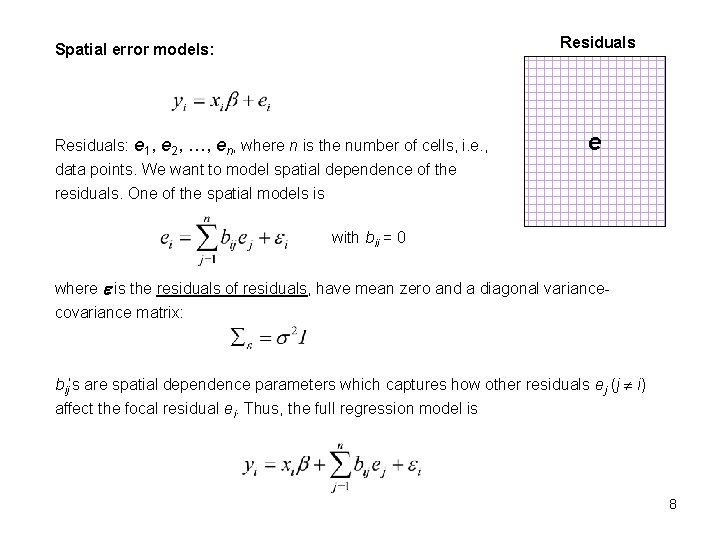
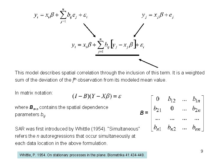
Residuals Spatial error models: Residuals: e 1, e 2, …, en, where n is the number of cells, i. e. , e data points. We want to model spatial dependence of the residuals. One of the spatial models is with bii = 0 where e is the residuals of residuals, have mean zero and a diagonal variancecovariance matrix: bij‘s are spatial dependence parameters which captures how other residuals ej (j i) affect the focal residual ei. Thus, the full regression model is 8

This model describes spatial correlation through the inclusion of this term. It is a weighted sum of the deviation of the jth observation from its modeled mean value. In matrix notation: where Bn n contains the spatial dependence parameters bij. B= SAR was first introduced by Whittle (1954). “Simultaneous” refers the n autoregressions that occur simultaneously at each data location in the above formulation. Whittle, P. 1954. On stationary processes in the plane. Biometrika 41: 434 -449. 9

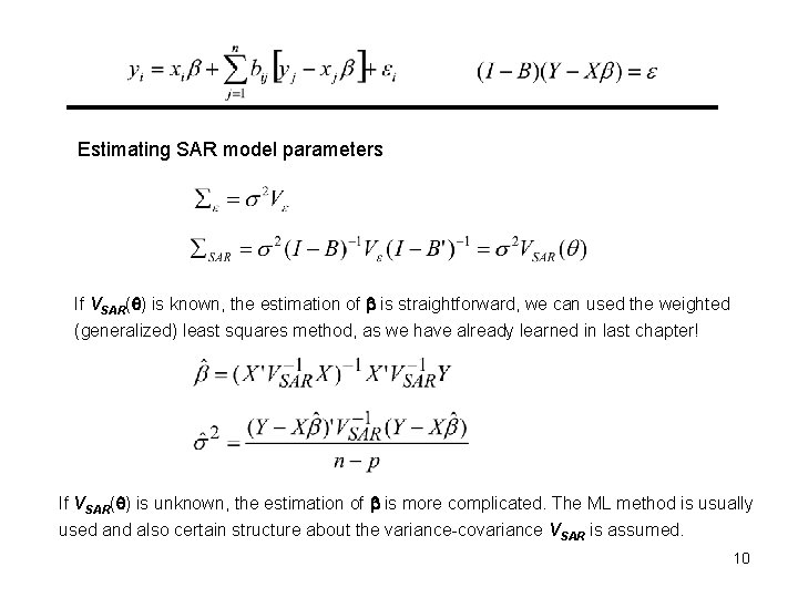
Estimating SAR model parameters If VSAR( ) is known, the estimation of b is straightforward, we can used the weighted (generalized) least squares method, as we have already learned in last chapter! If VSAR( ) is unknown, the estimation of b is more complicated. The ML method is usually used and also certain structure about the variance-covariance VSAR is assumed. 10

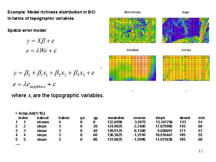
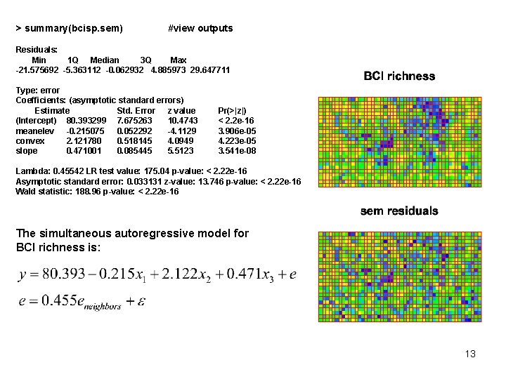
Example: Model richness distribution in BCI In terms of topographic variables. Spatial error model: where xi are the topographic variables. > bcisp. dat[1: 10, ] index habcat 1 1 stream 2 2 slope 3 3 slope 4 4 slope 5 5 slope …. habno 4 3 3 gx 0 0 0 gy 0 20 40 60 80 meanelev 122. 6950 124. 9025 128. 9125 130. 3825 131. 8025 convex -3. 5975 -2. 2460 -0. 1260 -1. 2910 -1. 5990 slope 13. 341756 17. 875906 9. 650691 10. 916467 11. 921838 abund 133 145 171 185 rich 54 60 57 55 60 11

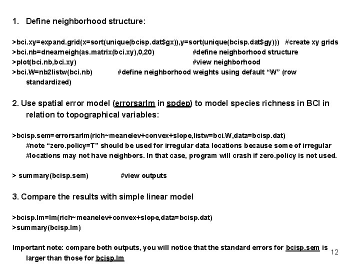
1. Define neighborhood structure: >bci. xy=expand. grid(x=sort(unique(bcisp. dat$gx)), y=sort(unique(bcisp. dat$gy))) #create xy grids >bci. nb=dnearneigh(as. matrix(bci. xy), 0, 20) #define neighborhood structure >plot(bci. nb, bci. xy) #view neighborhood >bci. W=nb 2 listw(bci. nb) #define neighborhood weights using default “W” (row standardized) 2. Use spatial error model (errorsarlm in spdep) to model species richness in BCI in relation to topographical variables: >bcisp. sem=errorsarlm(rich~meanelev+convex+slope, listw=bci. W, data=bcisp. dat) #note “zero. policy=T” should be used for irregular data locations because some of irregular #locations may not have neighbors. In that case, program will crash if zero. policy is not used. > summary(bcisp. sem) #view outputs 3. Compare the results with simple linear model >bcisp. lm=lm(rich~meanelev+convex+slope, data=bcisp. dat) >summary(bcisp. lm) Important note: compare both outputs, you will notice that the standard errors for bcisp. sem is 12 larger than those for bcisp. lm

> summary(bcisp. sem) #view outputs Residuals: Min 1 Q Median 3 Q Max -21. 575692 -5. 363112 -0. 062932 4. 885973 29. 647711 Type: error Coefficients: (asymptotic standard errors) Estimate Std. Error z value (Intercept) 80. 393299 7. 675263 10. 4743 meanelev -0. 215075 0. 052292 -4. 1129 convex 2. 121780 0. 518145 4. 0949 slope 0. 471001 0. 085445 5. 5123 Pr(>|z|) < 2. 2 e-16 3. 906 e-05 4. 223 e-05 3. 541 e-08 Lambda: 0. 45542 LR test value: 175. 04 p-value: < 2. 22 e-16 Asymptotic standard error: 0. 033131 z-value: 13. 746 p-value: < 2. 22 e-16 Wald statistic: 188. 96 p-value: < 2. 22 e-16 The simultaneous autoregressive model for BCI richness is: 13

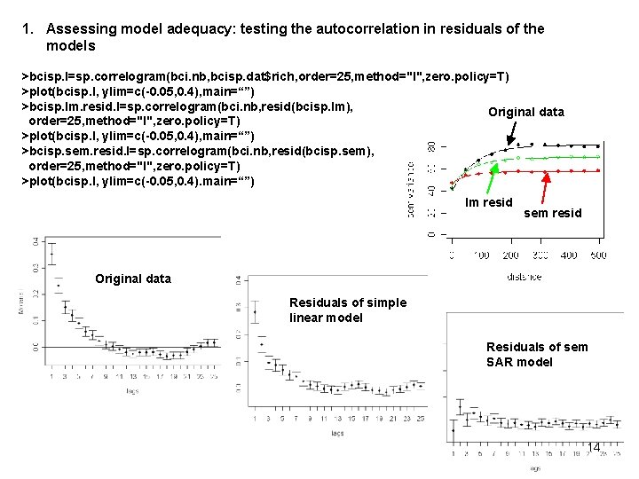
1. Assessing model adequacy: testing the autocorrelation in residuals of the models >bcisp. I=sp. correlogram(bci. nb, bcisp. dat$rich, order=25, method="I", zero. policy=T) >plot(bcisp. I, ylim=c(-0. 05, 0. 4), main=“”) >bcisp. lm. resid. I=sp. correlogram(bci. nb, resid(bcisp. lm), Original data order=25, method="I", zero. policy=T) >plot(bcisp. I, ylim=c(-0. 05, 0. 4), main=“”) >bcisp. sem. resid. I=sp. correlogram(bci. nb, resid(bcisp. sem), order=25, method="I", zero. policy=T) >plot(bcisp. I, ylim=c(-0. 05, 0. 4). main=“”) lm resid sem resid Original data Residuals of simple linear model Residuals of sem SAR model 14

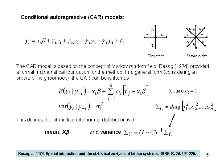
Conditional autoregressive (CAR) models: g 3 g 2 g 1 g 2 First-order g 1 g 4 g 1 g 2 g 3 Second-order The CAR model is based on the concept of Markov random field. Besag (1974) provided a formal mathematical foundation for the method. In a general form (considering all orders of neighborhood), the CAR can be written as Require cii = 0 This defines a joint multivariate normal distribution with mean: Xb and variance Besag, J. 1974, Spatial interaction and the statistical analysis of lattice systems. JRSS, B. 36: 192 -225. 15

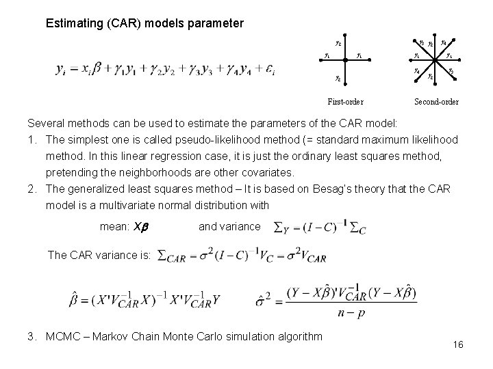
Estimating (CAR) models parameter g 3 g 2 g 1 g 2 First-order g 1 g 4 g 1 g 2 g 3 Second-order Several methods can be used to estimate the parameters of the CAR model: 1. The simplest one is called pseudo-likelihood method (= standard maximum likelihood method. In this linear regression case, it is just the ordinary least squares method, pretending the neighborhoods are other covariates. 2. The generalized least squares method – It is based on Besag’s theory that the CAR model is a multivariate normal distribution with mean: Xb and variance The CAR variance is: 3. MCMC – Markov Chain Monte Carlo simulation algorithm 16

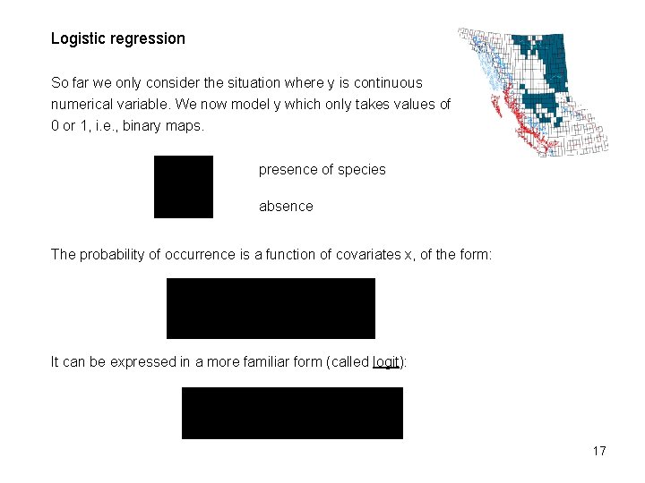
Logistic regression So far we only consider the situation where y is continuous numerical variable. We now model y which only takes values of 0 or 1, i. e. , binary maps. presence of species absence The probability of occurrence is a function of covariates x, of the form: It can be expressed in a more familiar form (called logit): 17

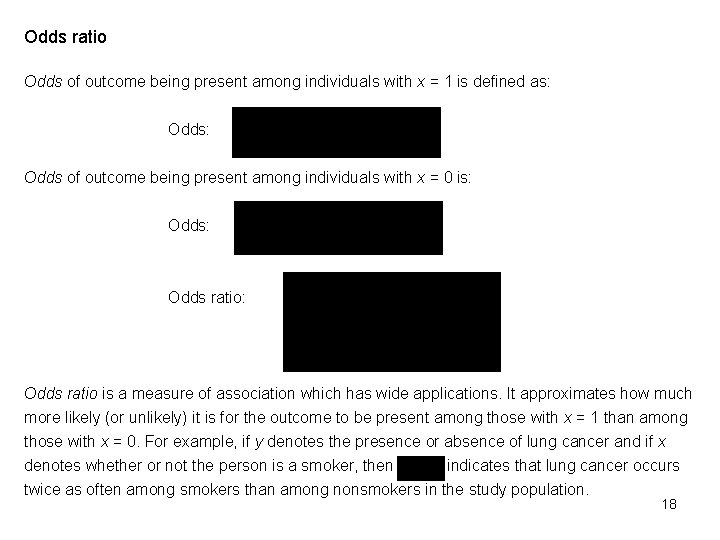
Odds ratio Odds of outcome being present among individuals with x = 1 is defined as: Odds of outcome being present among individuals with x = 0 is: Odds: Odds ratio is a measure of association which has wide applications. It approximates how much more likely (or unlikely) it is for the outcome to be present among those with x = 1 than among those with x = 0. For example, if y denotes the presence or absence of lung cancer and if x denotes whether or not the person is a smoker, then indicates that lung cancer occurs twice as often among smokers than among nonsmokers in the study population. 18

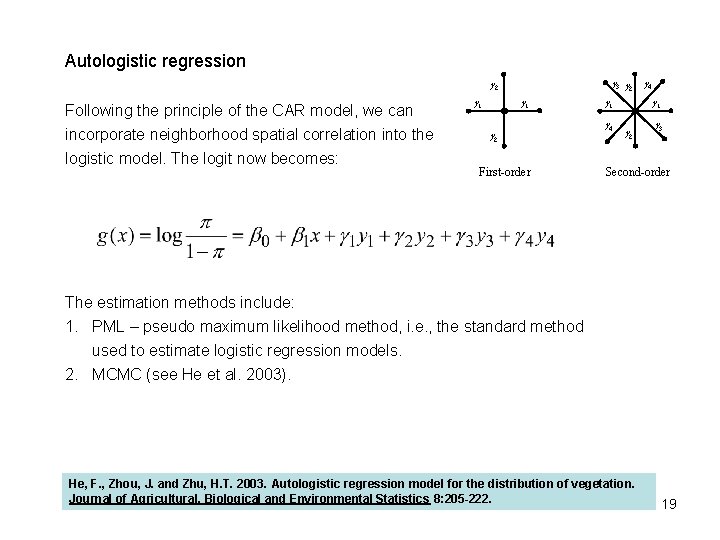
Autologistic regression g 3 g 2 Following the principle of the CAR model, we can incorporate neighborhood spatial correlation into the logistic model. The logit now becomes: g 1 g 2 First-order g 1 g 4 g 1 g 2 g 3 Second-order The estimation methods include: 1. PML – pseudo maximum likelihood method, i. e. , the standard method used to estimate logistic regression models. 2. MCMC (see He et al. 2003). He, F. , Zhou, J. and Zhu, H. T. 2003. Autologistic regression model for the distribution of vegetation. Journal of Agricultural, Biological and Environmental Statistics 8: 205 -222. 19

Spatial statistical analysis in Ecology 1. Point pattern analysis 2. Geostatistics 3. Lattice data analysis (regression) 1. Methods for testing (detecting) spatial structures/scale effect: (1) Quadrat methods, distance methods, Ripley’s K function (2) Moran’s I, Geary’s c (3) Geostatistic methods: variogram, covariogram 2. Saptial interpolation: naïve methods and kriging 3. Model lattice data: spatial autoregressive models 20