CHAPTER 11 Coping with NPcompleteness Algorithm 11 1

CHAPTER 11 Coping with NP-completeness

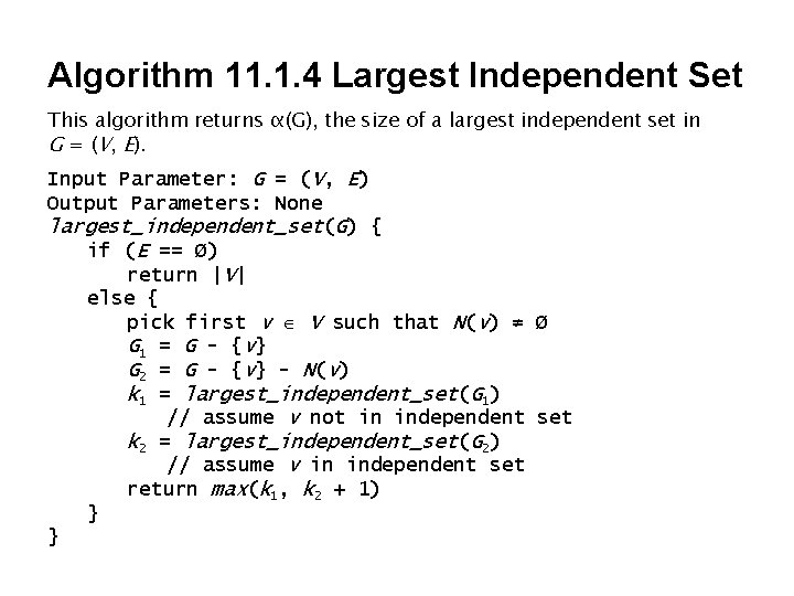
Algorithm 11. 1. 4 Largest Independent Set This algorithm returns α(G), the size of a largest independent set in G = (V, E). Input Parameter: G = (V, E) Output Parameters: None largest_independent_set(G) { if (E == Ø) return |V| else { pick first v V such that N(v) ≠ Ø G 1 = G - { v} G 2 = G - { v} - N(v) k 1 = largest_independent_set(G 1) // assume v not in independent set k 2 = largest_independent_set(G 2) // assume v in independent set return max(k 1, k 2 + 1) } }

Algorithm 11. 1. 11 3 -Satisfiability This algorithm takes as an input a formula in CNF in which every clause contains at most three literals and returns true if and only if is satisfiable.

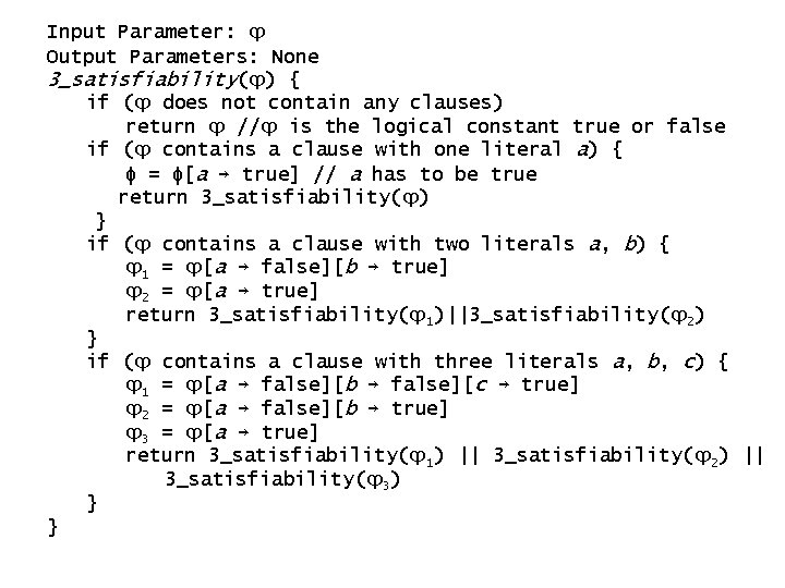
Input Parameter: ϕ Output Parameters: None 3_satisfiability(ϕ) { if (ϕ does not contain any clauses) return ϕ //ϕ is the logical constant true or false if (ϕ contains a clause with one literal a) { ϕ = ϕ[a → true] // a has to be true return 3_satisfiability(ϕ) } if (ϕ contains a clause with two literals a, b) { ϕ 1 = ϕ[a → false][b → true] ϕ 2 = ϕ[a → true] return 3_satisfiability(ϕ 1)||3_satisfiability(ϕ 2) } if (ϕ contains a clause with three literals a, b, c) { ϕ 1 = ϕ[a → false][b → false][c → true] ϕ 2 = ϕ[a → false][b → true] ϕ 3 = ϕ[a → true] return 3_satisfiability(ϕ 1) || 3_satisfiability(ϕ 2) || 3_satisfiability(ϕ 3) } }

Algorithm 11. 2. 1 Randomized st-Connectivity This algorithm takes as an input a graph G = (V, E) and two vertices s, t V. It returns true with probability one if there is a path from s to t; if there is no path from s to t, it fails to terminate. Input Parameters: G, s, t Output Parameters: None randomized_st_connectivity(G, s, t) { vertex = s while (vertex != t) vertex = random vertex from N(vertex) return true }

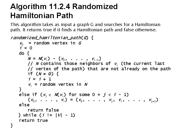
Algorithm 11. 2. 4 Randomized Hamiltonian Path This algorithm takes as input a graph G and searches for a Hamiltonian path. It returns true if it finds a Hamiltonian path and false otherwise. randomized_hamiltonian_path(G) { v 0 = random vertex in G i = 0 do { N = N(vi) - {v 0, . . . , vi-1} // N contains those neighbors of vi (the current last // vertex of the path) that are not already on the path if (N ≠ Ø) { i = i + 1 vi = random vertex in N } else if (vj N(vi) for some 0 = j < i - 1) (v 0, . . . , vi) = (v 0, . . . , vj, vi, . . . , vj+1) else return false } while (i != |V| - 1) return true }

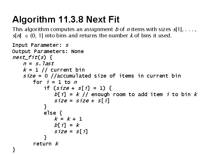
Algorithm 11. 3. 8 Next Fit This algorithm computes an assignment b of n items with sizes s[1], . . . , s[n] (0, 1] into bins and returns the number k of bins it used. Input Parameter: s Output Parameters: None next_fit(s) { n = s. last k = 1 // current bin size = 0 //accumulated size of items in current bin for i = 1 to n if (size + s[i] = 1) { b[i] = k // enough room to add item i to bin k size = size + s[i] } else { k = k + 1 b[i] = k size = s[i] } return k }

Algorithm 11. 3. 13 First Fit This algorithm computes an assignment b of n items with sizes s[1], . . . , s[n] (0, 1] into bins and returns the number k of bins it used.

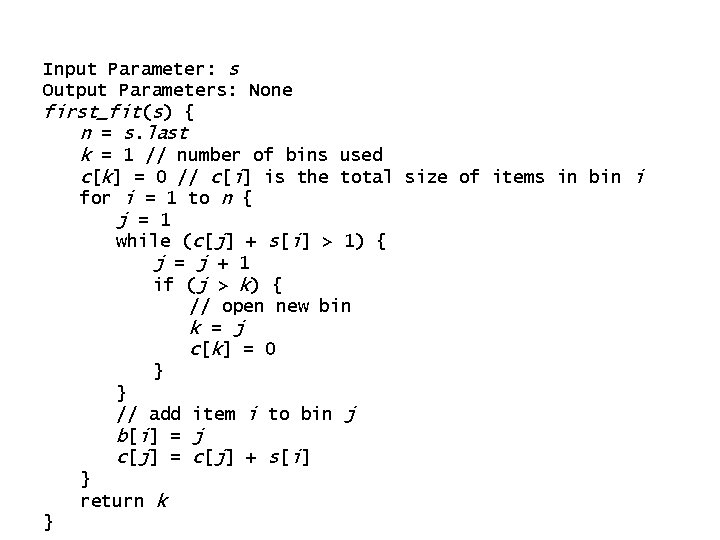
Input Parameter: s Output Parameters: None first_fit(s) { n = s. last k = 1 // number of bins used c[k] = 0 // c[i] is the total size of items in bin i for i = 1 to n { j = 1 while (c[j] + s[i] > 1) { j = j + 1 if (j > k) { // open new bin k = j c[k] = 0 } } // add item i to bin j b[i] = j c[j] = c[j] + s[i] } return k }

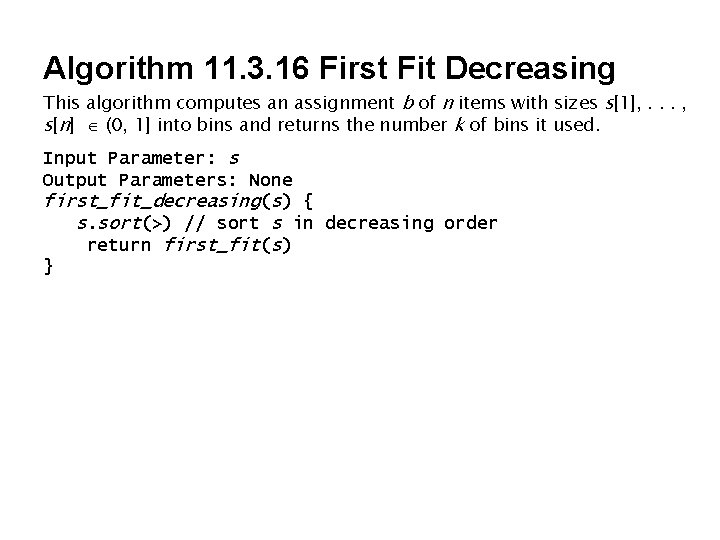
Algorithm 11. 3. 16 First Fit Decreasing This algorithm computes an assignment b of n items with sizes s[1], . . . , s[n] (0, 1] into bins and returns the number k of bins it used. Input Parameter: s Output Parameters: None first_fit_decreasing(s) { s. sort(>) // sort s in decreasing order return first_fit(s) }

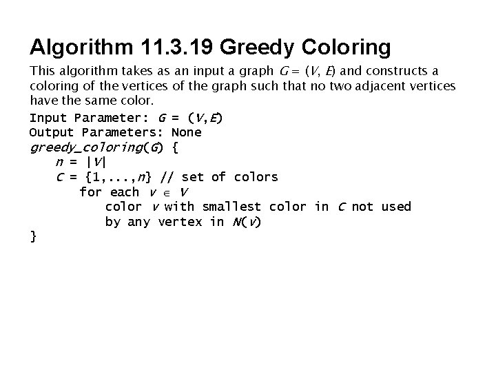
Algorithm 11. 3. 19 Greedy Coloring This algorithm takes as an input a graph G = (V, E) and constructs a coloring of the vertices of the graph such that no two adjacent vertices have the same color. Input Parameter: G = (V, E) Output Parameters: None greedy_coloring(G) { n = | V| C = {1, . . . , n} // set of colors for each v V color v with smallest color in C not used by any vertex in N(v) }

Algorithm 11. 3. 23 Wigderson Coloring This algorithm takes as input a 3 -colorable graph G = (V, E) and constructs a coloring of the vertices of the graph such that no two adjacent vertices have the same color.

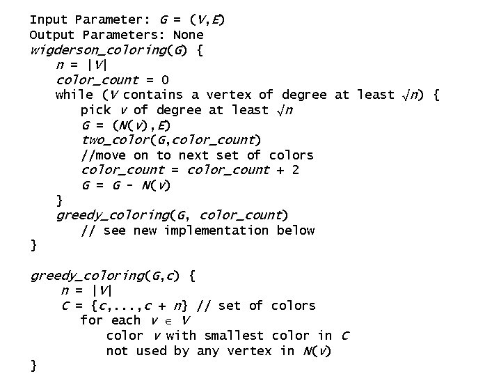
Input Parameter: G = (V, E) Output Parameters: None wigderson_coloring(G) { n = | V| color_count = 0 while (V contains a vertex of degree at least √n) { pick v of degree at least √n G = (N(v), E) two_color(G, color_count) //move on to next set of colors color_count = color_count + 2 G = G - N(v) } greedy_coloring(G, color_count) // see new implementation below } greedy_coloring(G, c) { n = | V| C = {c, . . . , c + n} // set of colors for each v V color v with smallest color in C not used by any vertex in N(v) }

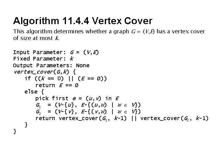
Algorithm 11. 4. 4 Vertex Cover This algorithm determines whether a graph G = (V, E) has a vertex cover of size at most k. Input Parameter: G = (V, E) Fixed Parameter: k Output Parameters: None vertex_cover(G, k) { if ((k == 0) || (E == Ø)) return E == Ø else { pick first e = (u, v) in E G 1 = (V-{u}, E-{(u, w) | w V}) G 2 = (V-{v}, E-{(v, w) | w V}) return vertex_cover(G 1, k-1) || vertex_cover(G 2, k-1) } }

Algorithm 11. 4. 7 Vertex Cover, Improved This algorithm determines whether a graph G = (V, E) has a vertex cover of size at most k.

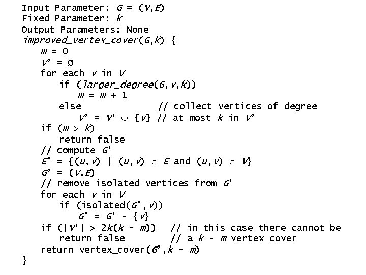
Input Parameter: G = (V, E) Fixed Parameter: k Output Parameters: None improved_vertex_cover(G, k) { m = 0 V’ = Ø for each v in V if (larger_degree(G, v, k)) m = m + 1 else // collect vertices of degree V’ = V’ {v} // at most k in V’ if (m > k) return false // compute G’ E’ = {(u, v) | (u, v) E and (u, v) V} G’ = ( V, E) // remove isolated vertices from G’ for each v in V if (isolated(G’, v)) G’ = G’ - { v} if (|V‘| > 2 k(k - m)) // in this case there cannot be return false // a k - m vertex cover return vertex_cover(G’, k - m) }

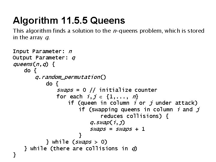
Algorithm 11. 5. 5 Queens This algorithm finds a solution to the n-queens problem, which is stored in the array q. Input Parameter: n Output Parameter: q queens(n, q) { do { q. random_permutation() do { swaps = 0 // initialize counter for each i, j {1, . . . , n} if (queen in column i or j under attack) if (swapping queens in column i and j reduces collisions) { q. swap(i, j) swaps = swaps + 1 } } while (swaps > 0) } while (there are collisions in q) }

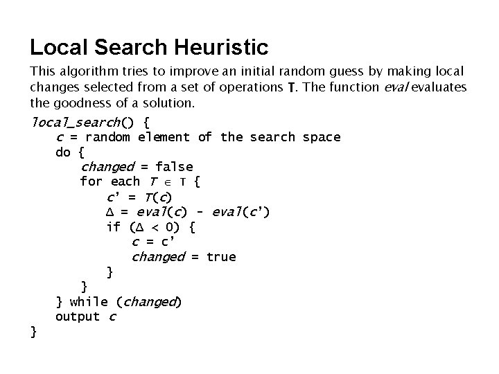
Local Search Heuristic This algorithm tries to improve an initial random guess by making local changes selected from a set of operations T. The function evaluates the goodness of a solution. local_search() { c = random element of the search space do { changed = false for each T T { c’ = T(c) Δ = eval(c) - eval(c’) if (Δ < 0) { c = c’ changed = true } } } while (changed) output c }

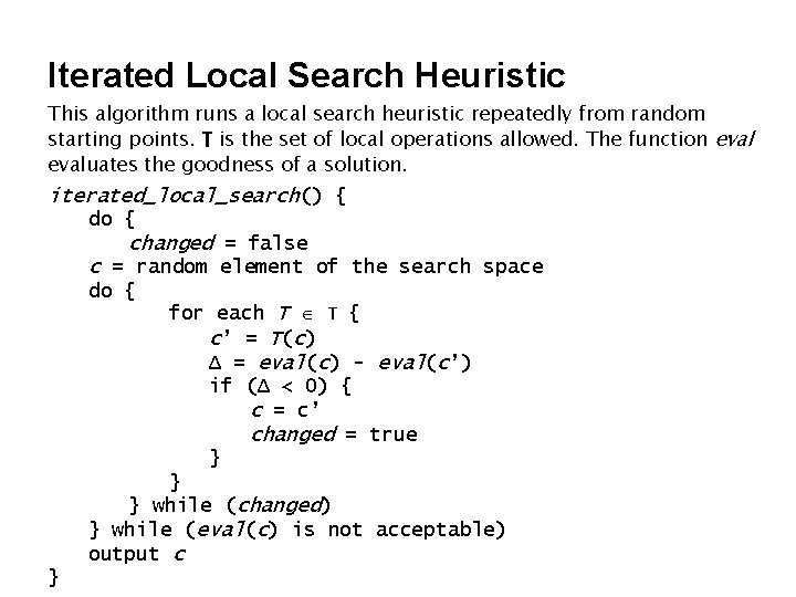
Iterated Local Search Heuristic This algorithm runs a local search heuristic repeatedly from random starting points. T is the set of local operations allowed. The function evaluates the goodness of a solution. iterated_local_search() { do { changed = false c = random element of the search space do { for each T T { c’ = T(c) Δ = eval(c) - eval(c’) if (Δ < 0) { c = c’ changed = true } } } while (changed) } while (eval(c) is not acceptable) output c }

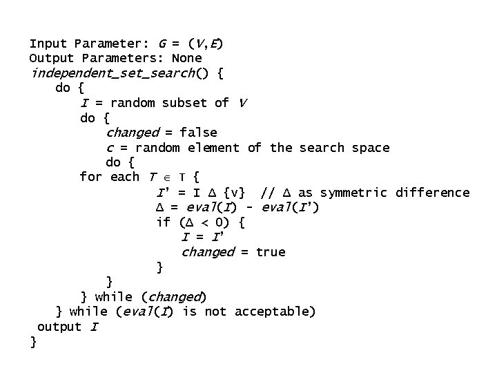
Algorithm 11. 5. 7 Independent Search This algorithm searches for a large independent set in the input graph G.

Input Parameter: G = (V, E) Output Parameters: None independent_search() { do { I = random subset of V do { changed = false c = random element of the search space do { for each T T { I’ = I Δ {v} // Δ as symmetric difference Δ = eval(I) - eval(I’) if (Δ < 0) { I = I’ changed = true } } } while (changed) } while (eval(I) is not acceptable) output I }

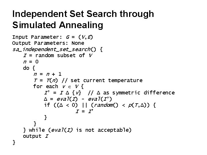
Independent Search through Simulated Annealing Input Parameter: G = (V, E) Output Parameters: None sa_independent_search() { I = random subset of V n = 0 do { n = n + 1 T = T(n) // set current temperature for each v V { I’ = I Δ {v} // Δ as symmetric difference Δ = eval(I) - eval(I’) if ((Δ < 0) || (random() < p(T, Δ)) { I = I’ } } } while (eval(I) is not acceptable) output I }