Appendix 4 A A Formal Model of Consumption

Appendix 4. A A Formal Model of Consumption and Saving © 2008 Pearson Addison-Wesley. All rights reserved

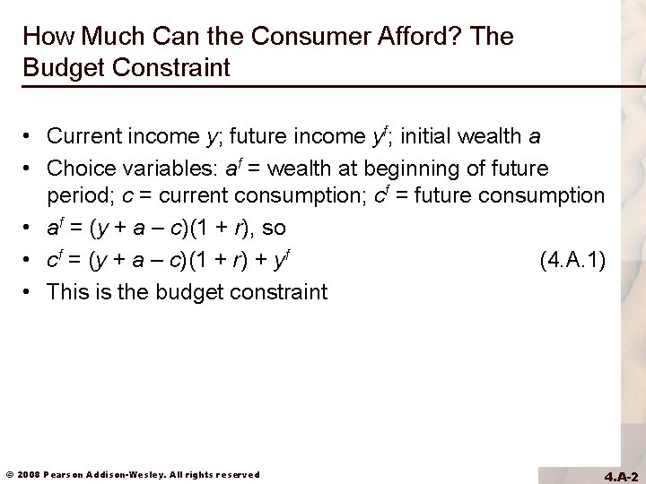
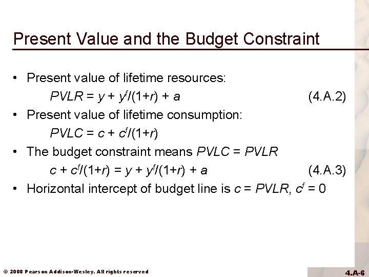
How Much Can the Consumer Afford? The Budget Constraint • Current income y; future income yf; initial wealth a • Choice variables: af = wealth at beginning of future period; c = current consumption; cf = future consumption • af = (y + a – c)(1 + r), so • cf = (y + a – c)(1 + r) + yf (4. A. 1) • This is the budget constraint © 2008 Pearson Addison-Wesley. All rights reserved 4. A-2

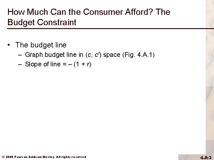
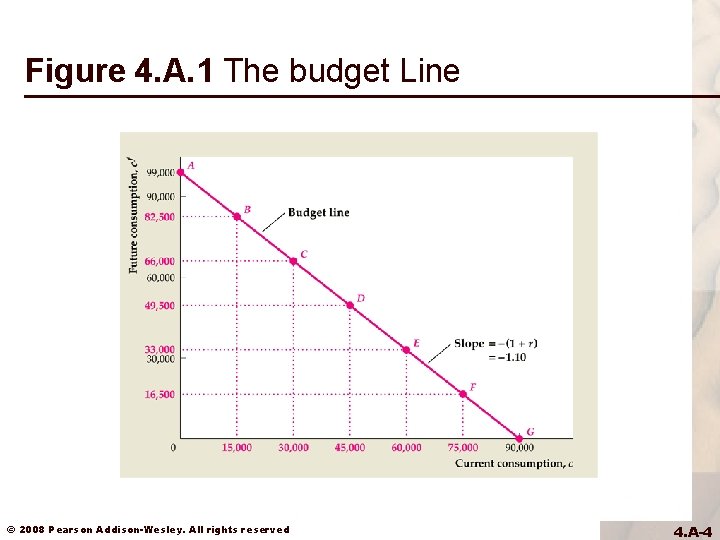
How Much Can the Consumer Afford? The Budget Constraint • The budget line – Graph budget line in (c, cf) space (Fig. 4. A. 1) – Slope of line = – (1 + r) © 2008 Pearson Addison-Wesley. All rights reserved 4. A-3

Figure 4. A. 1 The budget Line © 2008 Pearson Addison-Wesley. All rights reserved 4. A-4

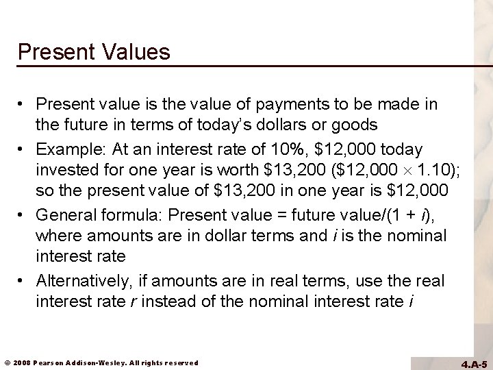
Present Values • Present value is the value of payments to be made in the future in terms of today’s dollars or goods • Example: At an interest rate of 10%, $12, 000 today invested for one year is worth $13, 200 ($12, 000 1. 10); so the present value of $13, 200 in one year is $12, 000 • General formula: Present value = future value/(1 + i), where amounts are in dollar terms and i is the nominal interest rate • Alternatively, if amounts are in real terms, use the real interest rate r instead of the nominal interest rate i © 2008 Pearson Addison-Wesley. All rights reserved 4. A-5

Present Value and the Budget Constraint • Present value of lifetime resources: PVLR = y + yf/(1+r) + a (4. A. 2) • Present value of lifetime consumption: PVLC = c + cf/(1+r) • The budget constraint means PVLC = PVLR c + cf/(1+r) = y + yf/(1+r) + a (4. A. 3) • Horizontal intercept of budget line is c = PVLR, cf = 0 © 2008 Pearson Addison-Wesley. All rights reserved 4. A-6

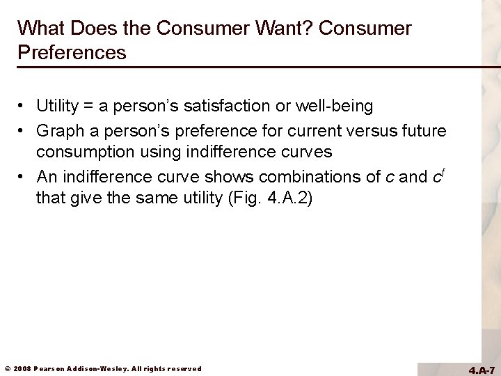
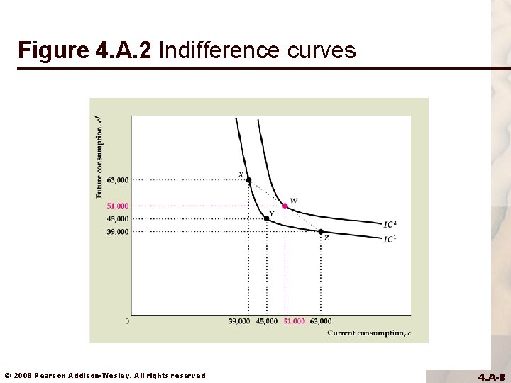
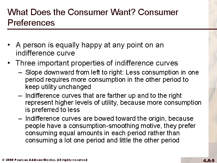
What Does the Consumer Want? Consumer Preferences • Utility = a person’s satisfaction or well-being • Graph a person’s preference for current versus future consumption using indifference curves • An indifference curve shows combinations of c and cf that give the same utility (Fig. 4. A. 2) © 2008 Pearson Addison-Wesley. All rights reserved 4. A-7

Figure 4. A. 2 Indifference curves © 2008 Pearson Addison-Wesley. All rights reserved 4. A-8

What Does the Consumer Want? Consumer Preferences • A person is equally happy at any point on an indifference curve • Three important properties of indifference curves – Slope downward from left to right: Less consumption in one period requires more consumption in the other period to keep utility unchanged – Indifference curves that are farther up and to the right represent higher levels of utility, because more consumption is preferred to less – Indifference curves are bowed toward the origin, because people have a consumption-smoothing motive, they prefer consuming equal amounts in each period rather than consuming a lot one period and little the other period © 2008 Pearson Addison-Wesley. All rights reserved 4. A-9

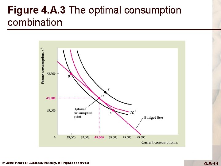
The Optimal Level of Consumption • Optimal consumption point is where the budget line is tangent to an indifference curve (Fig. 4. A. 3) • That’s the highest indifference curve that it’s possible to reach • All other points on the budget line are on lower indifference curves © 2008 Pearson Addison-Wesley. All rights reserved 4. A-10

Figure 4. A. 3 The optimal consumption combination © 2008 Pearson Addison-Wesley. All rights reserved 4. A-11

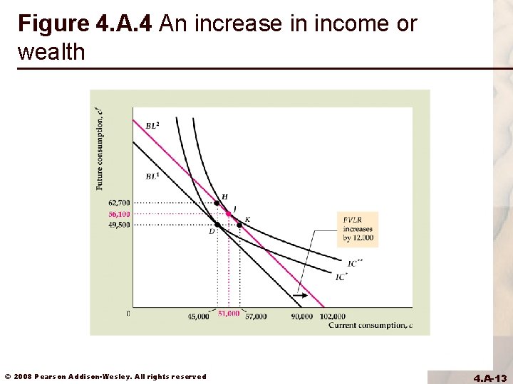
The Effects of Changes in Income and Wealth on Consumption and Saving • The effect on consumption of a change in income (current or future) or wealth depends only on how the change affects the PVLR – An increase in current income (Fig. 4. A. 4) • Increases PVLR, so shifts budget line out parallel to old budget line • If there is a consumption-smoothing motive, both current and future consumption will increase • Then both consumption and saving rise because of the rise in current income © 2008 Pearson Addison-Wesley. All rights reserved 4. A-12

Figure 4. A. 4 An increase in income or wealth © 2008 Pearson Addison-Wesley. All rights reserved 4. A-13

The Effects of Changes in Income and Wealth on Consumption and Saving • The effect on consumption of a change in income (current or future) or wealth depends only on how the change affects the PVLR – An increase in future income • Same outward shift in budget line as an increase in current income • Again, with consumption smoothing, both current and future consumption increase • Now saving declines, since current income is unchanged and current consumption increases – An increase in wealth • Same parallel shift in budget line, so both current and future consumption rise • Again, saving declines, since c rises and y is unchanged © 2008 Pearson Addison-Wesley. All rights reserved 4. A-14

The Effects of Changes in Income and Wealth on Consumption and Saving • The permanent income theory – Different types of changes in income • Temporary increase in income: y rises and yf is unchanged • Permanent increase in income: Both y and yf rise © 2008 Pearson Addison-Wesley. All rights reserved 4. A-15

The Effects of Changes in Income and Wealth on Consumption and Saving • The permanent income theory – Permanent income increase causes bigger increase in PVLR than a temporary income increase • So current consumption will rise more with a permanent income increase • So saving from a permanent increase in income is less than from a temporary increase in income © 2008 Pearson Addison-Wesley. All rights reserved 4. A-16

The Effects of Changes in Income and Wealth on Consumption and Saving • The permanent income theory – This distinction between permanent and temporary income changes was made by Milton Friedman in the 1950 s and is known as the permanent income theory • Permanent changes in income lead to much larger changes in consumption • Thus permanent income changes are mostly consumed, while temporary income changes are mostly saved © 2008 Pearson Addison-Wesley. All rights reserved 4. A-17

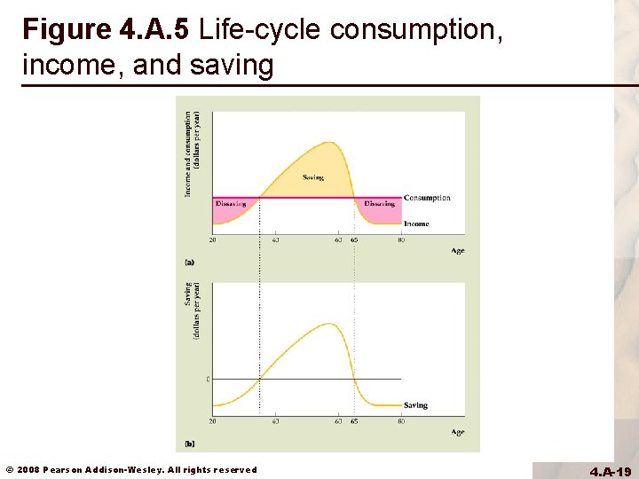
Consumption and Saving Over Many Periods: The Life-Cycle Model • Life-cycle model was developed by Franco Modigliani and associates in the 1950 s – Looks at patterns of income, consumption, and saving over an individual’s lifetime – Typical consumer’s income and saving pattern shown in Fig. 4. A. 5 © 2008 Pearson Addison-Wesley. All rights reserved 4. A-18

Figure 4. A. 5 Life-cycle consumption, income, and saving © 2008 Pearson Addison-Wesley. All rights reserved 4. A-19

Consumption and Saving Over Many Periods: The Life-Cycle Model • Real income steadily rises over time until near retirement; at retirement, income drops sharply • Lifetime pattern of consumption is much smoother than the income pattern – In reality, consumption varies somewhat by age – For example, when raising children, household consumption is higher than average – The model can easily be modified to handle this and other variations © 2008 Pearson Addison-Wesley. All rights reserved 4. A-20

Consumption and Saving Over Many Periods: The Life-Cycle Model • Saving has the following lifetime pattern – Saving is low or negative early in working life – Maximum saving occurs when income is highest (ages 50 to 60) – Dissaving occurs in retirement © 2008 Pearson Addison-Wesley. All rights reserved 4. A-21

Consumption and Saving Over Many Periods: The Life-Cycle Model • Bequests and saving – What effect does a bequest motive (a desire to leave an inheritance) have on saving? – Simply consume less and save more than without a bequest motive © 2008 Pearson Addison-Wesley. All rights reserved 4. A-22

Consumption and Saving Over Many Periods: The Life-Cycle Model • Ricardian equivalence – We can use the two-period model to examine Ricardian equivalence – The two-period model shows that consumption is changed only if the PVLR changes – Suppose the government reduces taxes by 100 in the current period, the interest rate is 10%, and taxes will be increased by 110 in the future period – Then the PVLR is unchanged, and thus there is no change in consumption © 2008 Pearson Addison-Wesley. All rights reserved 4. A-23

Consumption and Saving Over Many Periods: The Life-Cycle Model • Excess sensitivity and borrowing constraints – Generally, theories about consumption, including the permanent income theory, have been supported by looking at real-world data – But some researchers have found that the data show that the impact of an income or wealth change is different than that implied by a change in the PVLR – There seems to be excess sensitivity of consumption to changes in current income • This could be due to short-sighted behavior • Or it could be due to borrowing constraints © 2008 Pearson Addison-Wesley. All rights reserved 4. A-24

Consumption and Saving Over Many Periods: The Life-Cycle Model • Excess sensitivity and borrowing constraints – Borrowing constraints mean people can’t borrow as much as they want Lenders may worry that a consumer won’t pay back the loan, so they won’t lend – If a person wouldn’t borrow anyway, the borrowing constraint is said to be nonbinding – But if a person wants to borrow and can’t, the borrowing constraint is binding © 2008 Pearson Addison-Wesley. All rights reserved 4. A-25

Consumption and Saving Over Many Periods: The Life-Cycle Model • Excess sensitivity and borrowing constraints – A consumer with a binding borrowing constraint spends all income and wealth on consumption • So an increase in income or wealth will be entirely spent on consumption as well • This causes consumption to be excessively sensitive to current income changes – How prevalent are borrowing constraints? Perhaps 20% to 50% of the U. S. population faces binding borrowing constraints © 2008 Pearson Addison-Wesley. All rights reserved 4. A-26

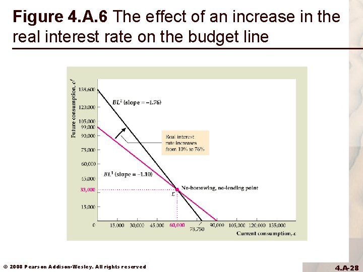
The Real Interest Rate and the Consumption. Saving Decision • The real interest rate and the budget line (Fig. 4. A. 6) – When the real interest rate rises, one point on the old budget line is also on the new budget line: the no-borrowing, nolending point – Slope of new budget line is steeper © 2008 Pearson Addison-Wesley. All rights reserved 4. A-27

Figure 4. A. 6 The effect of an increase in the real interest rate on the budget line © 2008 Pearson Addison-Wesley. All rights reserved 4. A-28

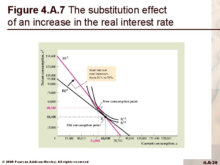
The Real Interest Rate and the Consumption. Saving Decision • The substitution effect – A higher real interest rate makes future consumption cheaper relative to current consumption – Increasing future consumption and reducing current consumption increases saving – Suppose a person is at the no-borrowing, no-lending point when the real interest rate rises (Fig. 4. A. 7) • An increase in the real interest rate unambiguously leads the person to increase future consumption and decrease current consumption • The increase in saving, equal to the decrease in current consumption, represents the substitution effect © 2008 Pearson Addison-Wesley. All rights reserved 4. A-29

Figure 4. A. 7 The substitution effect of an increase in the real interest rate © 2008 Pearson Addison-Wesley. All rights reserved 4. A-30

The Real Interest Rate and the Consumption. Saving Decision • The income effect – If a person is planning to consume at the no-borrowing, nolending point, then a rise in the real interest rate leads just to a substitution effect – But if a person is planning to consume at a different point than the no-borrowing, no-lending point, there is also an income effect © 2008 Pearson Addison-Wesley. All rights reserved 4. A-31

The Real Interest Rate and the Consumption. Saving Decision • The income effect – The intuition of the income effect • If the person originally planned to be a lender, the rise in the real interest rate gives the person more income in the future period; the income effect works in the opposite direction of the substitution effect, since more future income increases current consumption • If the person originally planned to be a borrower, the rise in the real interest rate gives the person less income in the future period; the income effect works in the same direction as the substitution effect, since less future income reduces current consumption further © 2008 Pearson Addison-Wesley. All rights reserved 4. A-32

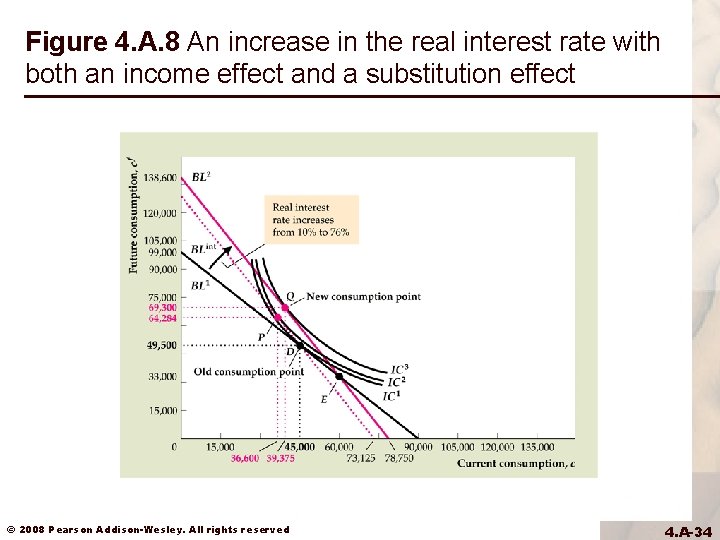
The Real Interest Rate and the Consumption. Saving Decision • The income and substitution effects together – Split the change in the budget line into two parts (Fig. 4. A. 8) – A budget line with the same slope as the new budget line, but going through the original consumption point (BLint) – The substitution effect is shown by the change from budget line BL 1 to budget line BLint, with the consumption point changing from point D to point P – The income effect is shown by the change from budget line BLint to budget line BL 2, with consumption point changing from point P to point Q © 2008 Pearson Addison-Wesley. All rights reserved 4. A-33

Figure 4. A. 8 An increase in the real interest rate with both an income effect and a substitution effect © 2008 Pearson Addison-Wesley. All rights reserved 4. A-34

The Real Interest Rate and the Consumption. Saving Decision • The income and substitution effects together – The substitution effect decreases current consumption, but the income effect increases current consumption; so saving may increase or decrease – Both effects increase future consumption – For a borrower, both effects decrease current consumption, so saving definitely increases but the effect on future consumption is ambiguous © 2008 Pearson Addison-Wesley. All rights reserved 4. A-35

The Real Interest Rate and the Consumption. Saving Decision • The income and substitution effects together – The effect on aggregate saving of a rise in the real interest rate is ambiguous theoretically • Empirical research suggests that saving increases • But the effect is small © 2008 Pearson Addison-Wesley. All rights reserved 4. A-36