Air pollutant emission impacts of electric vehicle market

Air pollutant emission impacts of electric vehicle market penetration scenarios Dan Loughlin, Samaneh Babaee*, Yang Ou*, Carol Lenox, Chris Nolte, and Tai Wu U. S. EPA Office of Research and Development * Research participants through the Oak Ridge Institute for Science and Education Susan Burke, Meredith Cleveland, Chris Ramig, Michael Shell, Ryan Sims, and Aaron Sobel U. S. EPA Office of Air and Radiation Steven J. Smith Joint Global Change Research Institute 1

Foreword • Intended audience • Air quality researchers and managers interested in assessing the multidecadal and environmental implications of emerging technologies and future scenarios. • Caveats • All results are intended to be illustrative. Assumptions are not fully described here. Please do not cite the results. • Acknowledgements • Others who have contributed substantially to the work presented here include Wenjing Shi, a grantee through the Oak Ridge Institute for Science and Education (ORISE), and Gokul Iyer of Pacific Northwest National Laboratory (PNNL). • Disclaimer • The views expressed in this presentation are those of the authors and do not necessarily represent the views or policies of the U. S. EPA or other author institutions. 2

Abbreviations • Models • GCAM – Global Change Assessment Model • GCAM-USA – GCAM version with state-level resolution for the United States • Emissions 3 • • • • BC – Black carbon CFCs - Chlorofluorocarbons CH 4 – Methane CO – Carbon monoxide CO 2 – Carbon dioxide GHG – Greenhouse gases N 2 O – Nitrous Oxide NOx – Nitrogen oxides OC – Organic carbon PM – Particulate Matter PM 2. 5 – PM of diameter less than 2. 5 microns SO 2 – Sulfur dioxide VOC – Volatile Organic Compounds • Units • EJ – Exajoules • MTC – Megatonnes Carbon • k. T – Kilotonnes • Technologies and fuels • • CCS – Carbon Capture and Sequestration CHP – Combined Heat and Power EV – Electric Vehicle CNG – Compressed Natural Gas • Organizations • • • JGCRI – Joint Global Change Research Institute NREL – National Renewable Energy Laboratory ORISE – Oak Ridge Institute for Science and Education PNNL – Pacific Northwest National Laboratory RGGI – Regional Greenhouse Gas Initiative U. S. EPA – United States Environmental Protection Agency • Other • • AEO 18 – Annual Energy Outlook 2018 PC – Personal Computer IPM – Integrated Planning Model GDP – Gross Domestic Product

Outline • Background • Human-earth system models • Global Change Assessment Model (GCAM) • GCAM Long-term Interactive Multi-Pollutant Scenario Evaluator (GLIMPSE) • Illustrative application: Electric vehicles • U. S. national impacts • U. S. regional impacts • Summary • Next steps 4

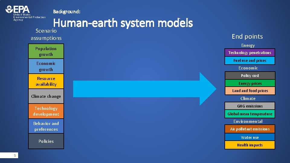
Background: Human-earth system models Scenario assumptions Population growth Economic growth Resource availability Climate change Technology development Behavior and preferences Policies 5 End points Energy Technology penetrations Fuel use and prices Economic Policy cost Energy prices Land food prices Climate GHG emissions Global mean temperature Environmental Air pollutant emissions Water use Health impacts

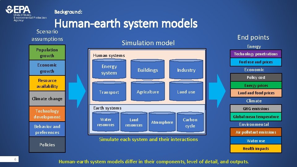
Background: Human-earth system models Scenario assumptions Simulation model Population growth Human systems Economic growth Energy system Resource availability End points Energy Technology penetrations Fuel use and prices Buildings Industry Policy cost Energy prices Transport Agriculture Land use Climate change Technology development Behavior and preferences Policies 6 Economic Land food prices Climate Earth systems Water resources GHG emissions Land resources Atmosphere Carbon cycle Global mean temperature Environmental Air pollutant emissions Simulate each system and their interactions Water use Health impacts Human-earth system models differ in their components, level of detail, and outputs.

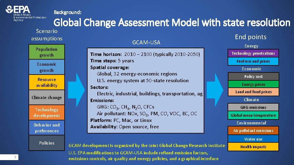
Background: Global Change Assessment Model with state resolution Scenario assumptions Population growth Economic growth Resource availability Climate change Technology development Behavior and preferences Policies 7 GCAM-USA Time horizon: 2010 – 2100 (typically 2010 -2050) Time steps: 5 years Spatial coverage: Global, 32 energy-economic regions U. S. energy system at 50 -state resolution Sectors: Electric, industrial, buildings, transportation, ag Emissions: GHG: CO 2, CH 4, N 2 O, CFCs Air pollutant: NOx, SO 2, PM, CO, VOC, BC, OC Platform: PC, Mac, or Linux Availability: Open source, free End points Energy Technology penetrations Fuel use and prices Economic Policy cost Energy prices Land food prices Climate GHG emissions Global mean temperature Environmental Air pollutant emissions Water use GCAM development is organized by the Joint Global Change Research Institute U. S. EPA modifications to GCAM-USA include refined emission factors, emissions controls, air quality and energy policies, and a graphical interface Health impacts

Background: Topics that can be explored with GCAM-USA • Estimate future air pollutant and greenhouse gas emissions • Evaluate outputs over alternative scenarios or assumptions • Population, GDP, technologies, etc. • Evaluate the impacts of various policies and regulations • • • Pollutant taxes or caps Renewable portfolio standards Vehicle efficiency standards Subsidies on specific technologies Emission standards on new sources • For various technological or policy scenarios • Characterize cross-sector interactions • Identify unintended consequences • Develop low-cost management strategies • Simultaneously considering measures such as controls, energy efficiency, renewable electricity, and fuel switching 8

Background: GLIMPSE multi-pollutant scenario evaluator Scenario assumptions Population growth Economic growth Resource availability Climate change Technology development Behavior and preferences Policies 9 GLIMPSE End points Energy Time horizon: 2010 – 2100 (typically 2010 -2050) Time steps: 5 years Spatial coverage: Global, 32 energy-economic regions U. S. energy system at 50 -state resolution Sectors: Electric, industrial, buildings, transportation Emissions: GHG: CO 2, CH 4, N 2 O, CFCs Air pollutant: NOx, SO 2, PM, CO, VOC, BC, OC Platform: PC, Mac, or Linux Availability: Open source, free Technology penetrations Fuel use and prices Economic Policy cost Energy prices Land food prices Climate GHG emissions Global mean temperature Environmental Air pollutant emissions Water use The GLIMPSE graphical interface simplifies setting up and executing modeling runs, visualizing results Health impacts

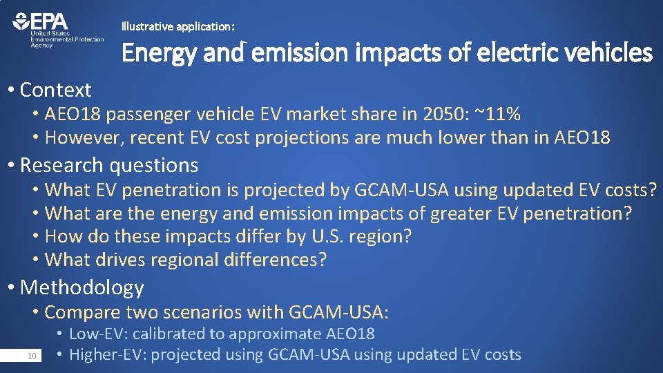
Illustrative application: Energy and emission impacts of electric vehicles • Context • AEO 18 passenger vehicle EV market share in 2050: ~11% • However, recent EV cost projections are much lower than in AEO 18 • Research questions • What EV penetration is projected by GCAM-USA using updated EV costs? • What are the energy and emission impacts of greater EV penetration? • How do these impacts differ by U. S. region? • What drives regional differences? • Methodology • Compare two scenarios with GCAM-USA: 10 • Low-EV: calibrated to approximate AEO 18 • Higher-EV: projected using GCAM-USA using updated EV costs

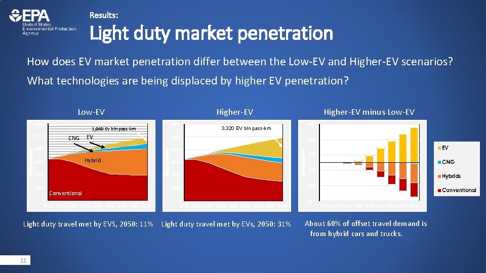
Results: Light duty market penetration How does EV market penetration differ between the Low-EV and Higher-EV scenarios? What technologies are being displaced by higher EV penetration? Low-EV CNG EV 8000 Hybrid 6000 4000 2000 Conventional 0 2015 2020 2025 2030 2035 2040 2045 2050 8000 6000 4000 2000 0 2015 2020 2025 2030 2035 2040 2045 2050 Light duty travel met by EVS, 2050: 11% Light duty travel met by EVs, 2050: 31% 11 2500 3, 320 EV bln pass-km 10000 Billion pass-km 10000 12000 1, 040 EV bln pass-km Higher-EV minus Low-EV 1500 Billion pass-km 12000 Higher-EV 500 -1500 -2500 2015 2020 2025 2030 2035 2040 2045 2050 About 60% of offset travel demand is from hybrid cars and trucks.

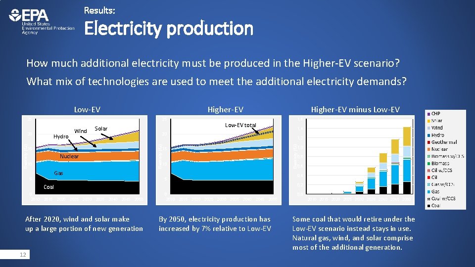
Results: Electricity production How much additional electricity must be produced in the Higher-EV scenario? What mix of technologies are used to meet the additional electricity demands? Low-EV Higher-EV 25 25 1, 6 Low-EV total 1, 4 20 15 Nuclear 10 1, 2 Electricity (EJ) Hydro Solar Electricity (EJ) 20 Wind Higher-EV minus Low-EV 15 10 Gas 5 2015 0, 6 0, 2 2020 2025 2030 2035 2040 2045 2050 After 2020, wind and solar make up a large portion of new generation 12 0, 8 0, 4 5 Coal 0 2010 1, 0 0 2010 0, 0 2015 2020 2025 2030 2035 2040 2045 2050 By 2050, electricity production has increased by 7% relative to Low-EV 2010 2015 2020 2025 2030 2035 2040 2045 2050 Some coal that would retire under the Low-EV scenario instead stays in use. Natural gas, wind, and solar comprise most of the additional generation.

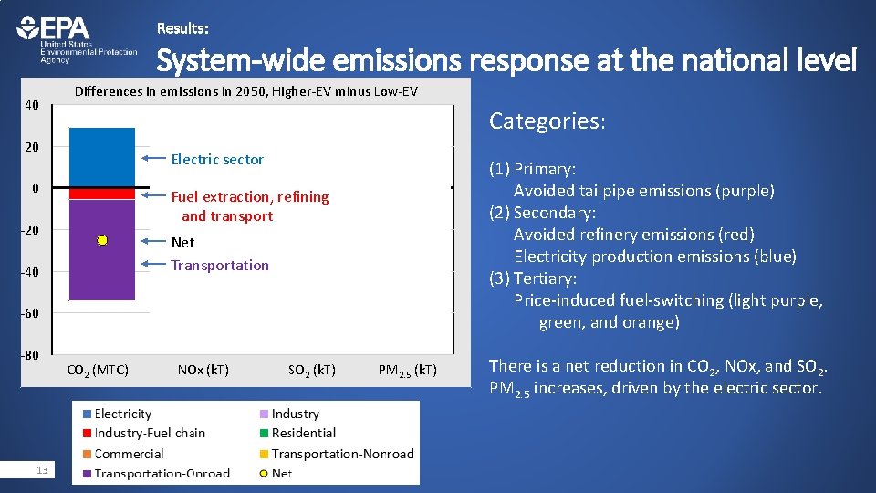
Results: System-wide emissions response at the national level 40 Differences in emissions in 2050, Higher-EV minus Low-EV Categories: 20 Electric sector 0 (1) Primary: Avoided tailpipe emissions (purple) (2) Secondary: Avoided refinery emissions (red) Electricity production emissions (blue) (3) Tertiary: Price-induced fuel-switching (light purple, green, and orange) Fuel extraction, refining and transport -20 Net Transportation -40 -60 -80 13 (MTC) COCO 2 2 (MTC) NOx (Kt) NOx (k. T) SO 2 SO(Kt) (k. T) 2 PM 2. 5 (Kt) PM 2. 5 (k. T) There is a net reduction in CO 2, NOx, and SO 2. PM 2. 5 increases, driven by the electric sector.

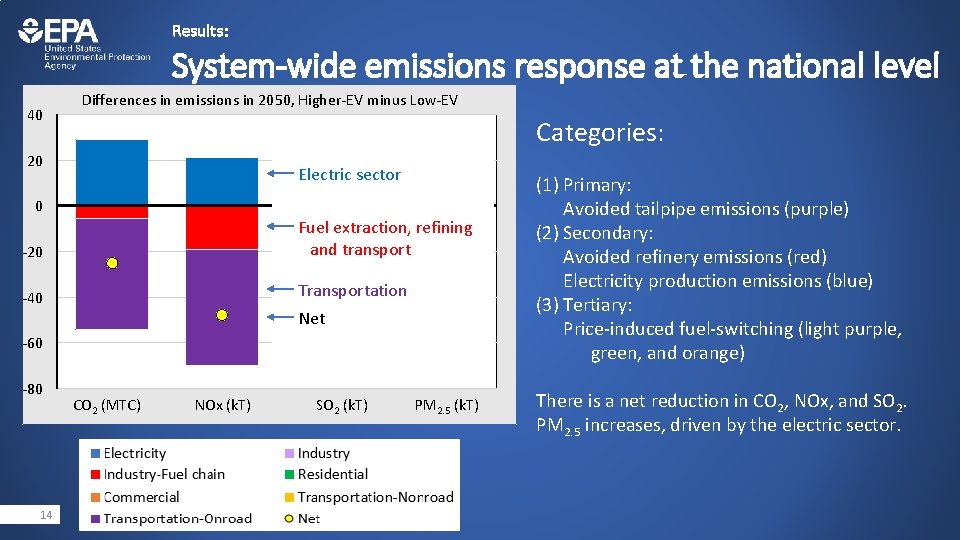
Results: System-wide emissions response at the national level 40 Differences in emissions in 2050, Higher-EV minus Low-EV Categories: 20 Electric sector 0 -20 Fuel extraction, refining and transport -40 Transportation Net -60 -80 14 (MTC) COCO 2 2 (MTC) NOx (Kt) NOx (k. T) SO 2 SO(Kt) (k. T) 2 PM 2. 5 (Kt) PM 2. 5 (k. T) (1) Primary: Avoided tailpipe emissions (purple) (2) Secondary: Avoided refinery emissions (red) Electricity production emissions (blue) (3) Tertiary: Price-induced fuel-switching (light purple, green, and orange) There is a net reduction in CO 2, NOx, and SO 2. PM 2. 5 increases, driven by the electric sector.

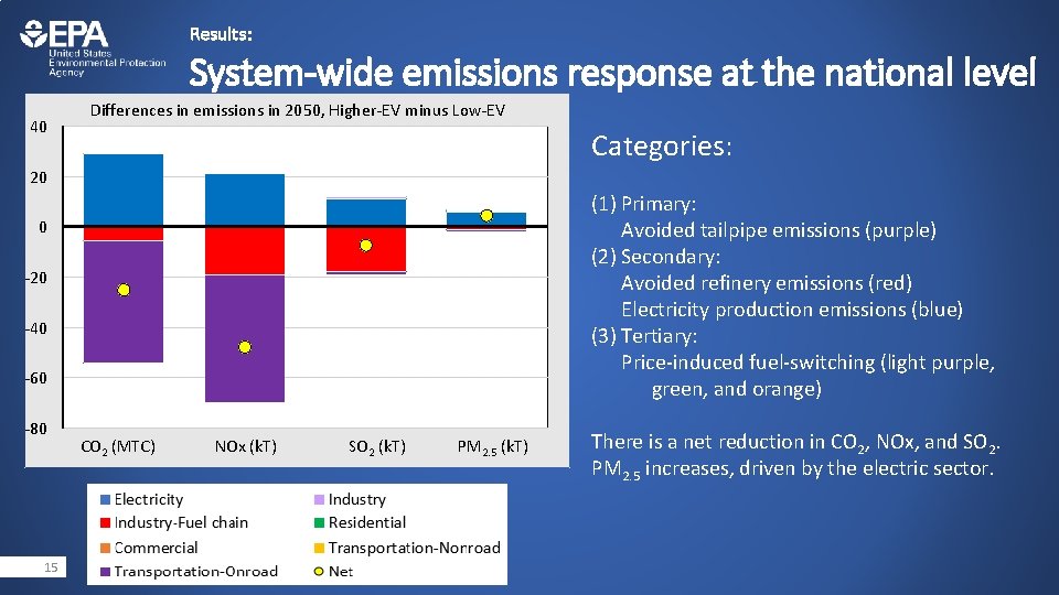
Results: System-wide emissions response at the national level 40 Differences in emissions in 2050, Higher-EV minus Low-EV Categories: 20 (1) Primary: Avoided tailpipe emissions (purple) (2) Secondary: Avoided refinery emissions (red) Electricity production emissions (blue) (3) Tertiary: Price-induced fuel-switching (light purple, green, and orange) 0 -20 -40 -60 -80 15 (MTC) COCO 2 2 (MTC) NOx (Kt) NOx (k. T) SO 2 SO(Kt) (k. T) 2 PM 2. 5 (Kt) PM 2. 5 (k. T) There is a net reduction in CO 2, NOx, and SO 2. PM 2. 5 increases, driven by the electric sector.

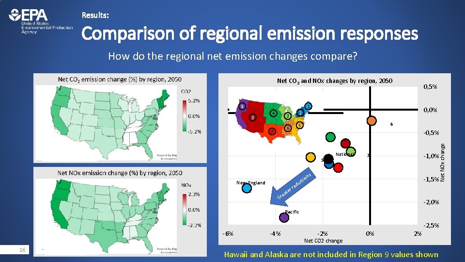
Results: Comparison of regional emission responses How do the regional net emission changes compare? Net CO 2 and NOx changes by region, 2050 9 8 4 2 3 7 1 0, 0% 6 5 6 0, 5% -0, 5% 4 5 New England 1 ate e Gr r c du re National 2 ns Net NOx change 8 -1, 0% 3 7 -1, 5% tio -2, 0% Pacific 9 -6% 16 -4% -2, 5% -2% Net CO 2 change 0% 2% Hawaii and Alaska are not included in Region 9 values shown

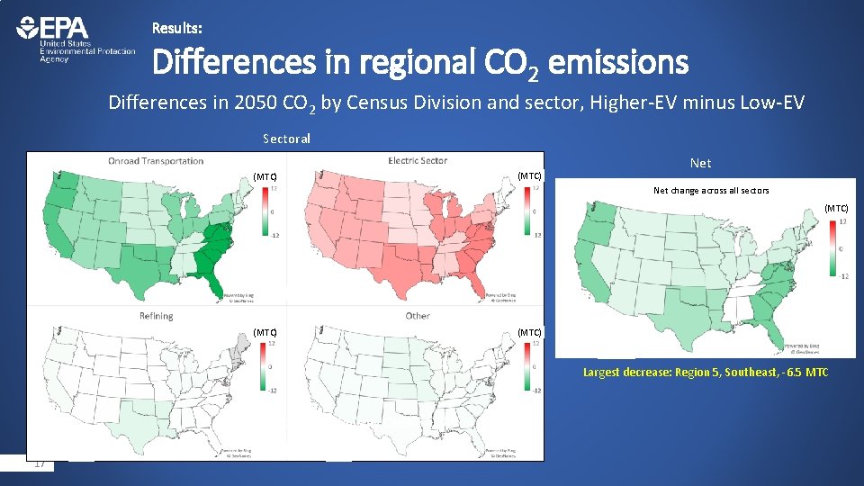
Results: Differences in regional CO 2 emissions Differences in 2050 CO 2 by Census Division and sector, Higher-EV minus Low-EV Sectoral (MTC) Net change across all sectors (MTC) Largest decrease: Region 5, Southeast, -6. 5 MTC Net change in CO 2 emissions by Census Division 17

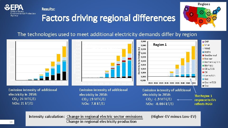
Regions Results: 9 Factors driving regional differences 4 8 7 3 6 2 5 The technologies used to meet additional electricity demands differ by region 0, 20 0, 08 0, 18 Electricity by technology (EJ) Region 6 0, 04 0, 02 0, 16 Region 9 (w/o Hawaii and Alaska) 0, 14 2010 2015 2020 2025 2030 2035 2040 2045 2050 Emission intensity of additional electricity in 2050: CO 2: 24 MTC/EJ NOx: 21 k. T/EJ 18 0, 040 0, 04 0, 03 0, 12 0, 10 RGGI Region 1 Region 0, 035 0, 030 0, 025 0, 020 0, 08 0, 06 0, 01 0, 04 0, 00 0, 02 0, 015 0, 010 0, 005 0, 000 0, 05 0, 045 Electricity by technology (EJ) 0, 10 -0, 02 2010 2015 2020 2025 2030 2035 2040 2045 2050 -0, 01 -0, 005 2010 2015 2020 2025 2030 2050 2025 20302035 2040 2045 2050 Emission intensity of additional electricity in 2050: CO 2: 19 MTC/EJ NOx: 7. 8 k. T/EJ Intensity calculation: Change in regional electric sector emissions Change in regional electricity production Emission intensity of additional electricity in 2050: CO 2: -1. 9 MTC/EJ NOx: -0. 004 k. T/EJ The Region 1 response to EVs reflects RGGI (Higher-EV minus Low-EV) 1

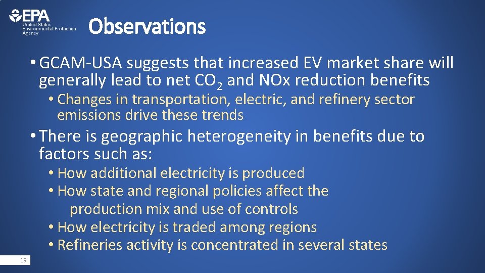
Observations • GCAM-USA suggests that increased EV market share will generally lead to net CO 2 and NOx reduction benefits • Changes in transportation, electric, and refinery sector emissions drive these trends • There is geographic heterogeneity in benefits due to factors such as: • How additional electricity is produced • How state and regional policies affect the production mix and use of controls • How electricity is traded among regions • Refineries activity is concentrated in several states 19

Summary • GCAM-USA can be applied to examine the long-term energy and emission impacts of EVs • Categories of impacts: • Primary (transportation sector) • Secondary (electricity production and refining) • Tertiary (price-induced fuel switching within and across sectors) • State-level insights informed by: • Existing technology stock • Fuel prices and renewable resources • State, regional, and national policies and regulations 20

Next Steps • Re-evaluate EV scenarios with the forthcoming version of GCAM-USA, which has an improved electric sector representation • Explore higher EV penetration scenarios • Link GCAM-USA with IPM to provide a more detailed exploration of electric sector response to EVs, including under alternative charging scenarios 21

Questions? For more information, please contact: Loughlin. Dan@epa. gov https: //www. epa. gov/air-research/glimpsecomputational-framework-supporting-state-levelenvironmental-and-energy 22