61 st OSU International Symposiumon Molecular Spectroscopy TH

61 st OSU International Symposiumon Molecular Spectroscopy TH 09 Analysis of interactions between excited vibrationalstates in the FASSST rotational spectrum of S(CN)2 Zbigniew Kisiel, Orest Dorosh Institute of Physics, Polish Academy of Sciences Ivan R. Medvedev, Marcus Behnke, Manfred Winnewisser, Frank C. De Lucia, Eric Herbst, Department of Physics, The Ohio State University

The challenge: FASSST mmw spectrum (see WI 04) continuous 110. 1 – 374. 3 GHz spectrum recorded at OSU at frequency accuracy of ca 50 k. Hz, resolution of 0. 5 -1 MHz, and containing >100000 measurable lines The solution: Computer packages for efficient data reduction = CAAARS (WI 04) and AABS http: //info. ifpan. edu. pl/~kisiel/prospe. htm

SVIEW_L = spectral viewer Name of data file for the fitting program Indicator of synchronized operation when Predictions for many spectroscopic species a single keystroke actions measurement can be displayed simultaneously and of line closest to prediction and adds the differentiated with various color, linestyle frequency and quantum numbers to the and highlighting dataset Synchronized Indicator of transition cursors and Name of predictions file already in the fitting frequency axes containing the current dataset Quantum numbers of the transition current transition (up to six per energy level) ASCP_L = viewer of predictions

Synthetic overview of the ground state dataset (nobs-ncalc)/dn, Red symbols denote (nobs-ncalc) > 3 dn Symbol size is proportional to:

Lowest energyvibrationalstates in S(CN)2 Frequencies are unscaled B 3 LYP/6 -31 G(d, p) w 3= 496 Other modes (cm-1): A 1 w 8= 366 w 9= 372 w 7= 328 B 1 w 4= 122 cm-1 A 1 B 2 A 2 n 6 n 5 n 1 G obs. calc. 672 685 A 1 690 688 B 1 2180 2293 B 1 2308 A 1

Loomis-Wood plot centered on. Ka = 1 - 0 transitions in the ground state 7 = 1 8 = 1 9 gs 4 = 1 =2 =3

4 = 3 9 = 1, Ka=1 - 0 Ka=2 - 1 Ka=3 - 2

Perturbations between 8 = 1 and 9 = 1 visible in. R-type transitions

Perturbations( 8 = R-type 1 9 = 1) and ( 8 = 1 4 = 3) Q-type

Hcor = i(Ga +…)Pa+ (Fbg +…) (Pb. Pg+Pg. Pb)… A 1 A 2= A 2 4 = 3 Rb: Fac+… (3 constants) 9 = 1 A 2 A 1 B 2= B 2 A 2 B 2= B 1 Ra: DE + Fbc+… (4 constants) 8 = 1 B 2 Rc: DE + Fab+… (8 constants) z(c) = 0 !

Plots of (1 -pmix) for energy levels in the interacting triad near 370 cm-1

Plots of obs-calc differences for measured rotational transitions in the 370 cm-1 triad

A 1 A 1= A 1 3 = 1 W 14 +… (3 constants) 4 = 4 A 1 Ra: DE + Fbc+… (4 constants) A 1 A 2= A 2 Rb: Fac+… (3 constants) B 2 … ) + = c nts 1 b A F ta + ns E o B 2 D : a 4 c ( R 8 = 1 4 = 1 B 2 A 2= A R: b 2 (3 c Fac + ons … tan ts) A 1 B 2= B 2 A 1 9 = 1 4 = 1 A 2 B 2= B 1 Rc: DE + Fab+… (8 constants) A 2

-1 (1 -pmix) plots for the interacting tetrad of states near 500 cm

-1 Obs-calc plots for the interacting tetrad of states near 500 cm

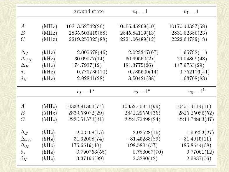
Assignment ofvibrationalsatellites (using relative intensity, statistical weights and inertial defects): calc (cm-1) G weight gs n 4 n 7 n 8 n 9 n 3 Inertial defect (u. A 2) obs. calc. 0. 49041(1) 0. 480 1. 38528(2) 1. 370 -0. 79070(3) -0. 852 122 323 A 1 B 1 + - 366 B 2 - 0. 71380(3) 0. 688 372 A 2 + 1. 00655(3) 1. 131 496 A 1 + 0. 95354(5) 0. 947 Weight denotes statistical weights relative to the ground state: + stands for unchanged - denotes reversed weights Reassigned Calc results from uscaled B 3 LYP/6 -31 G(d, p)

Vibrational energy differences resulting from coupled fits triad near 370 cm-1: tetrad near 500 cm-1 :

Conclusions: FASSST spectrum of S(CN)2 assigned, over 18000 lines measured analysed resulting in: Precise constants for the ground state and all 11 different vibrational excited states of the parent isotopomer for vibrational energy up to ca 500 cm-1 Constants for ground states of 34 S and 13 C isotopomers Deviations of fits from 50 to 100 k. Hz Confident assignment of first excited states of five different normal modes Many precise vibrational energy level differences + … Creation of highly efficient AABS software package in order to manage data for many states simultaneously

Updated