ya Sp MV Yet Another Sp MV Framework

ya. Sp. MV: Yet Another Sp. MV Framework on GPUs Shengen Yan, Chao Li, Yunquan Zhang, Huiyang Zhou 1

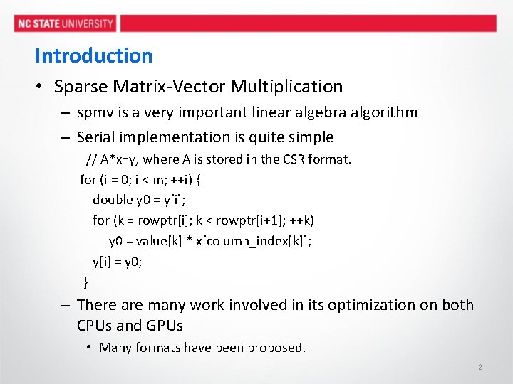
Introduction • Sparse Matrix-Vector Multiplication – spmv is a very important linear algebra algorithm – Serial implementation is quite simple // A*x=y, where A is stored in the CSR format. for (i = 0; i < m; ++i) { double y 0 = y[i]; for (k = rowptr[i]; k < rowptr[i+1]; ++k) y 0 = value[k] * x[column_index[k]]; y[i] = y 0; } – There are many work involved in its optimization on both CPUs and GPUs • Many formats have been proposed. 2

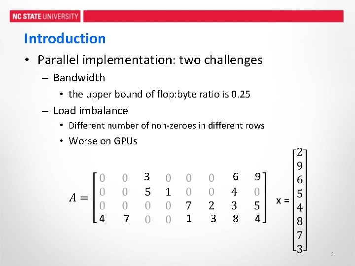
Introduction • Parallel implementation: two challenges – Bandwidth • the upper bound of flop: byte ratio is 0. 25 – Load imbalance • Different number of non-zeroes in different rows • Worse on GPUs 3 4 7 1 3 6 9 8 4 3

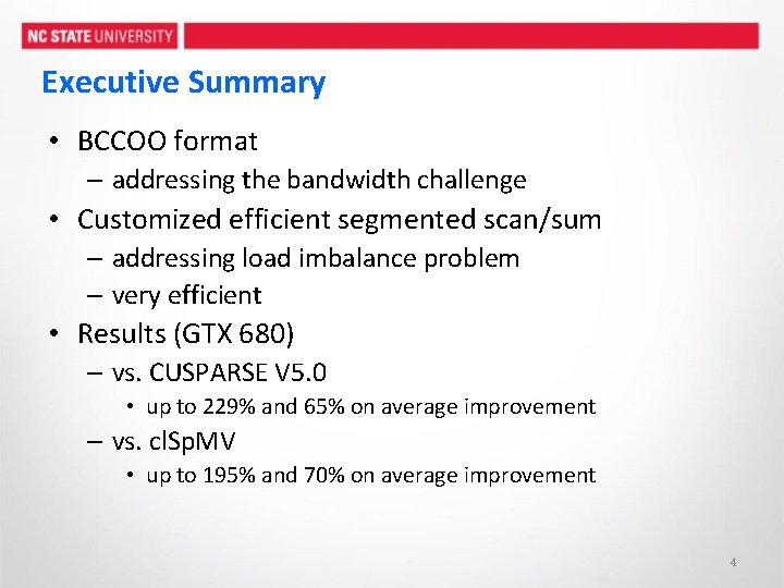
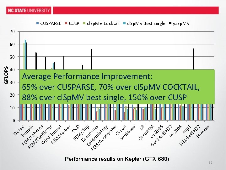
Executive Summary • BCCOO format – addressing the bandwidth challenge • Customized efficient segmented scan/sum – addressing load imbalance problem – very efficient • Results (GTX 680) – vs. CUSPARSE V 5. 0 • up to 229% and 65% on average improvement – vs. cl. Sp. MV • up to 195% and 70% on average improvement 4

Outline • Introduction • Formats for Sp. MV – addressing the bandwidth challenge • • Efficient Segmented Sum/Scan for Sp. MV Auto-Tuning Framework Experimentation Conclusions 5

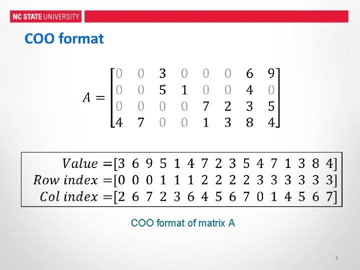
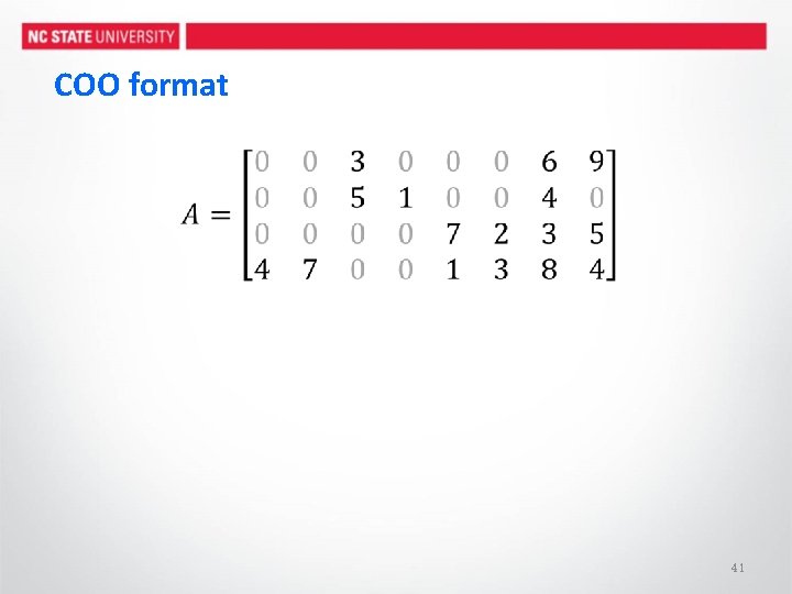
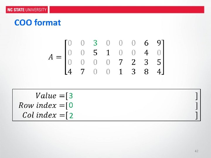
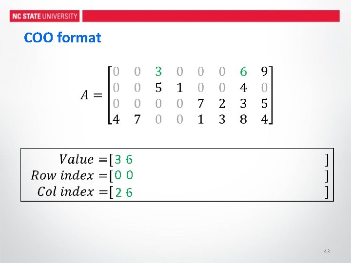
COO format of matrix A 6

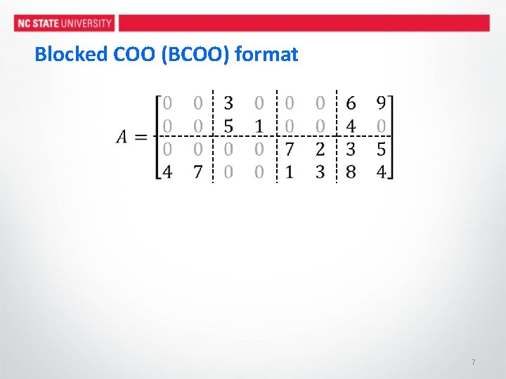
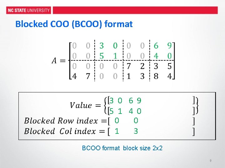
Blocked COO (BCOO) format 7

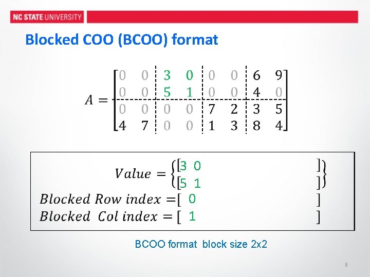
Blocked COO (BCOO) format 3 0 5 1 0 1 BCOO format block size 2 x 2 8

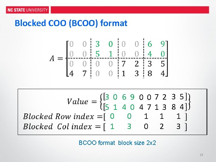
Blocked COO (BCOO) format 3 0 6 9 5 1 4 0 0 0 1 3 BCOO format block size 2 x 2 9

Blocked COO (BCOO) format 3 0 6 9 0 07 2 3 5 5 1 4 0 4 71 3 8 4 0 0 1 1 3 0 2 3 BCOO format block size 2 x 2 10

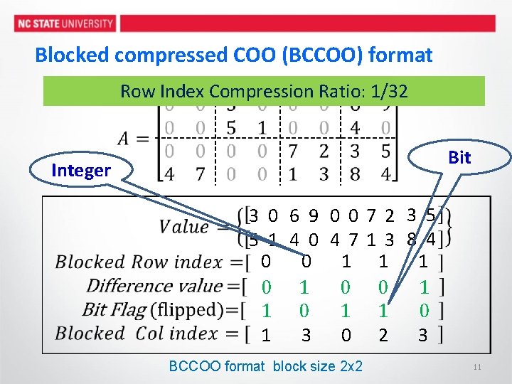
Blocked compressed COO (BCCOO) format Row Index Compression Ratio: 1/32 Bit Integer 3 0 6 9 0 07 2 3 5 5 1 4 0 4 71 3 8 4 0 0 1 1 1 0 0 1 1 0 1 3 0 2 3 BCCOO format block size 2 x 2 11

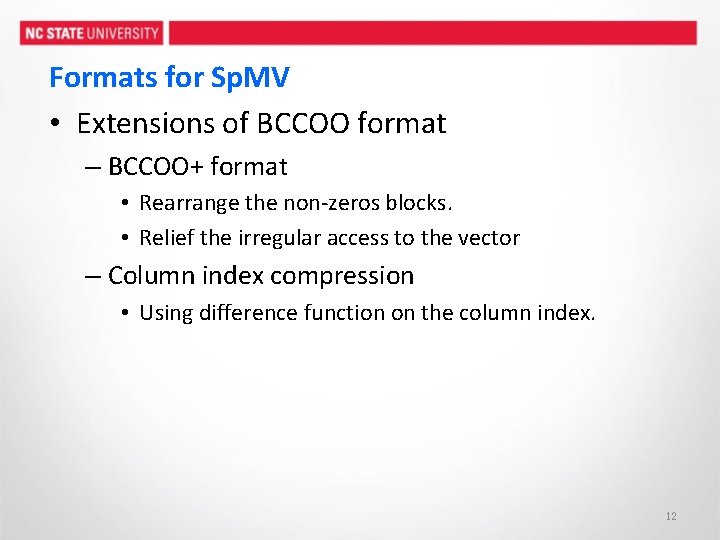
Formats for Sp. MV • Extensions of BCCOO format – BCCOO+ format • Rearrange the non-zeros blocks. • Relief the irregular access to the vector – Column index compression • Using difference function on the column index. 12

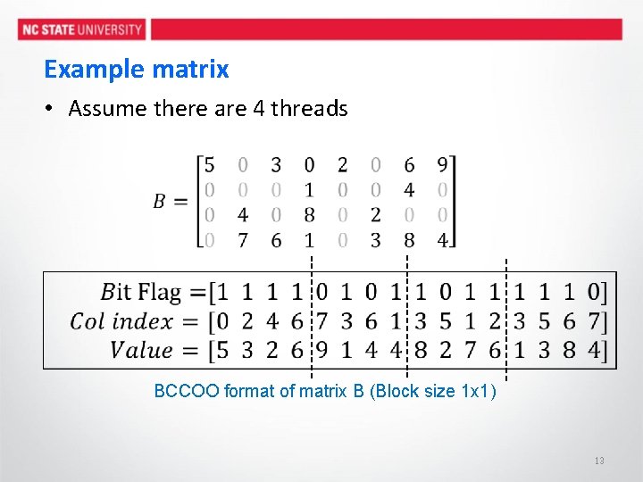
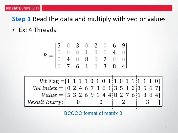
Example matrix • Assume there are 4 threads BCCOO format of matrix B (Block size 1 x 1) 13

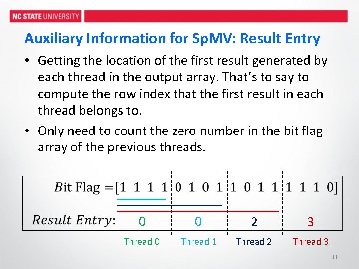
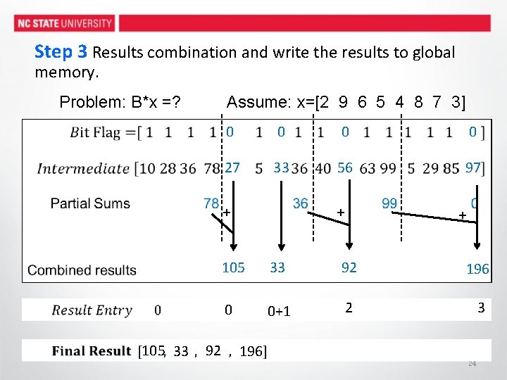
Auxiliary Information for Sp. MV: Result Entry • Getting the location of the first result generated by each thread in the output array. That’s to say to compute the row index that the first result in each thread belongs to. • Only need to count the zero number in the bit flag array of the previous threads. 0 0 2 3 Thread 0 Thread 1 Thread 2 Thread 3 14

Outline • Introduction • Formats for Sp. MV • Efficient Segmented Sum/Scan for Sp. MV – addressing load imbalance problem • Auto-Tuning Framework • Experimentation • Conclusions 15

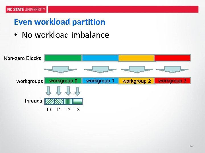
Even workload partition • No workload imbalance Non-zero Blocks workgroup 0 workgroup 1 workgroup 2 workgroup 3 threads T 0 T 1 T 2 T 3 16

Efficient Segmented Sum/Scan for Sp. MV • Three logic steps – Read the data and multiply them with the corresponding vector values. – Perform a segmented sum/scan using the bit flag array from our BCCOO/BCCOO+ format – Results combination and write back the results to global memory. • All these three steps are implemented in one kernel 17

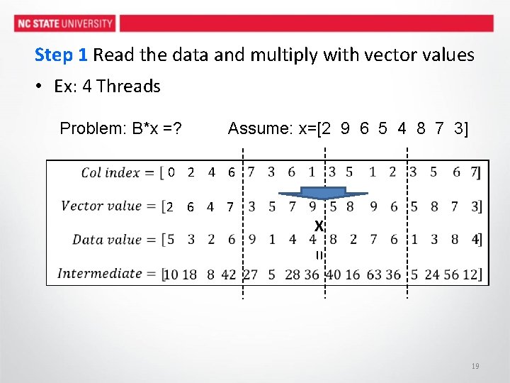
Step 1 Read the data and multiply with vector values • Ex: 4 Threads BCCOO format of matrix B 18

Step 1 Read the data and multiply with vector values • Ex: 4 Threads Problem: B*x =? Assume: x=[2 9 6 5 4 8 7 3] 0 2 4 6 2 6 4 7 X = 19

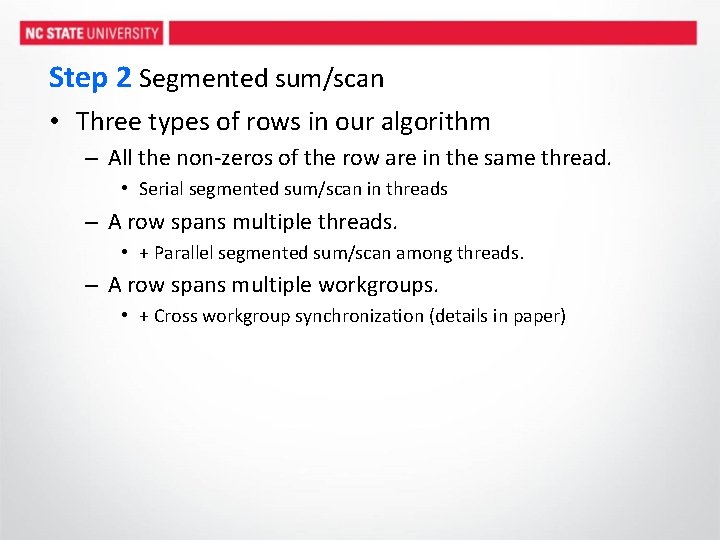
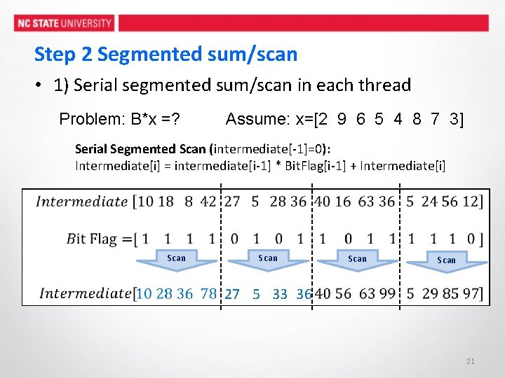
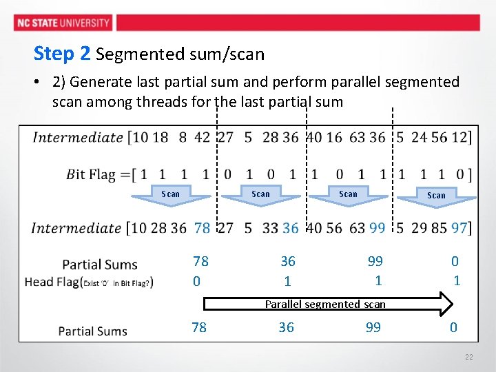
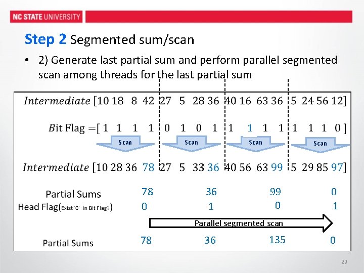
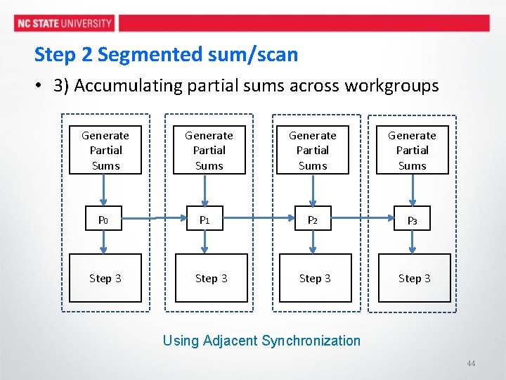
Step 2 Segmented sum/scan • Three types of rows in our algorithm – All the non-zeros of the row are in the same thread. • Serial segmented sum/scan in threads – A row spans multiple threads. • + Parallel segmented sum/scan among threads. – A row spans multiple workgroups. • + Cross workgroup synchronization (details in paper)

Step 2 Segmented sum/scan • 1) Serial segmented sum/scan in each thread Problem: B*x =? Assume: x=[2 9 6 5 4 8 7 3] Serial Segmented Scan (intermediate[-1]=0): Intermediate[i] = intermediate[i-1] * Bit. Flag[i-1] + Intermediate[i] Scan 27 5 33 36 21

Step 2 Segmented sum/scan • 2) Generate last partial sum and perform parallel segmented scan among threads for the last partial sum Scan 78 0 Scan 36 1 Scan 99 1 0 1 Parallel segmented scan 78 36 99 0 22

Step 2 Segmented sum/scan • 2) Generate last partial sum and perform parallel segmented scan among threads for the last partial sum 1 Scan 78 0 Scan 36 1 Scan 99 0 1 Parallel segmented scan 78 36 135 99 0 23

Step 3 Results combination and write the results to global memory. Assume: x=[2 9 6 5 4 8 7 3] Problem: B*x =? 0 0 27 33 56 97 + 105 33 92 + + 105 33 92 196 0 0+1 2 3 196 24

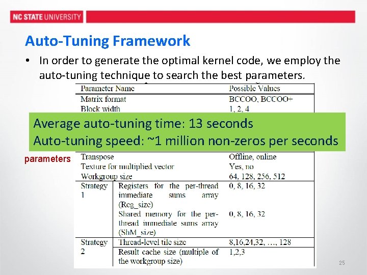
Auto-Tuning Framework • In order to generate the optimal kernel code, we employ the auto-tuning technique to search the best parameters. Average auto-tuning time: 13 seconds Auto-tuning speed: ~1 million non-zeros per seconds Tunable parameters 25

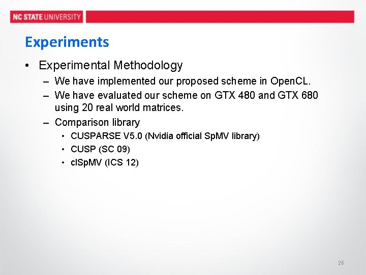
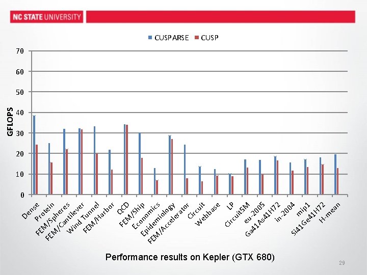
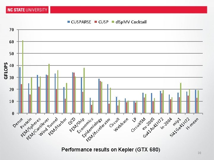
Experiments • Experimental Methodology – We have implemented our proposed scheme in Open. CL. – We have evaluated our scheme on GTX 480 and GTX 680 using 20 real world matrices. – Comparison library • CUSPARSE V 5. 0 (Nvidia official Sp. MV library) • CUSP (SC 09) • cl. Sp. MV (ICS 12) 26

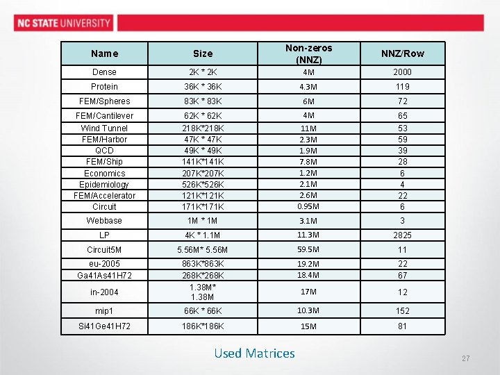
Name Size Non-zeros (NNZ) NNZ/Row Dense 2 K * 2 K 4 M 2000 Protein 36 K * 36 K 4. 3 M 119 FEM/Spheres 83 K * 83 K 6 M 72 FEM/Cantilever 62 K * 62 K 4 M 65 Wind Tunnel FEM/Harbor QCD FEM/Ship Economics Epidemiology FEM/Accelerator Circuit 218 K*218 K 47 K * 47 K 49 K * 49 K 141 K*141 K 207 K*207 K 526 K*526 K 121 K*121 K 171 K*171 K 11 M 2. 3 M 1. 9 M 7. 8 M 1. 2 M 2. 1 M 2. 6 M 0. 95 M 53 59 39 28 6 4 22 6 Webbase 1 M * 1 M 3 LP 4 K * 1. 1 M 11. 3 M 2825 Circuit 5 M 5. 56 M* 5. 56 M 59. 5 M 11 eu-2005 Ga 41 As 41 H 72 863 K*863 K 268 K*268 K 1. 38 M* 1. 38 M 19. 2 M 18. 4 M 22 67 17 M 12 mip 1 66 K * 66 K 10. 3 M 152 Si 41 Ge 41 H 72 186 K*186 K 15 M 81 in-2004 Used Matrices 27

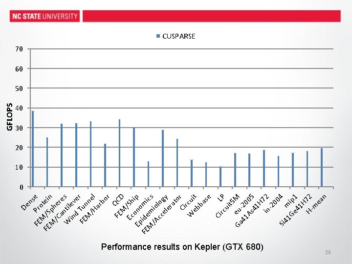
FE n Pr se M o FE /S tein M ph /C er a e W ntil s in ev d e FE Tun r M n /H el ar bo r Q FE CD M Ec /Sh Ep ono ip FE ide mi M m cs /A io cc log el y er at o Ci r W rcui eb t ba se Ci rc LP ui t 5 Ga eu M 41 -20 As 05 41 H in 72 -2 00 4 Si 4 m 1 G ip e 4 1 1 H H- 72 m ea n De GFLOPS CUSPARSE 70 60 50 40 30 20 10 0 Performance results on Kepler (GTX 680) 28

FE n Pr se M o FE /S tein M ph /C er a e W ntil s in ev d e FE Tun r M n /H el ar bo r Q FE CD M Ec /Sh Ep ono ip FE ide mi M m cs /A io cc log el y er at o Ci r W rcui eb t ba se Ci rc LP ui t 5 Ga eu M 41 -20 As 05 41 H in 72 -2 00 4 Si 4 m 1 G ip e 4 1 1 H H- 72 m ea n De GFLOPS CUSPARSE CUSP 70 60 50 40 30 20 10 0 Performance results on Kepler (GTX 680) 29

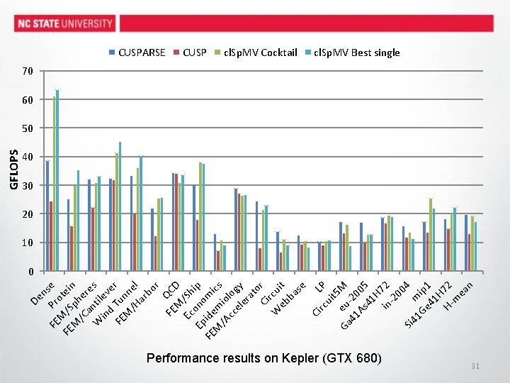
FE n Pr se M o FE /S tein M ph /C er a e W ntil s in ev d e FE Tun r M n /H el ar bo r Q FE CD M Ec /Sh Ep ono ip FE ide mi M m cs /A io cc log el y er at o Ci r W rcui eb t ba se Ci rc LP ui t 5 Ga eu M 41 -20 As 05 41 H in 72 -2 00 4 Si 4 m 1 G ip e 4 1 1 H H- 72 m ea n De GFLOPS CUSPARSE CUSP cl. Sp. MV Cocktail 70 60 50 40 30 20 10 0 Performance results on Kepler (GTX 680) 30

FE n Pr se M o FE /S tein M ph /C er a e W ntil s in ev d e FE Tun r M n /H el ar bo r Q FE CD M Ec /Sh Ep ono ip FE ide mi M m cs /A io cc log el y er at o Ci r W rcui eb t ba se Ci rc LP ui t 5 Ga eu M 41 -20 As 05 41 H in 72 -2 00 4 Si 4 m 1 G ip e 4 1 1 H H- 72 m ea n De GFLOPS CUSPARSE CUSP cl. Sp. MV Cocktail cl. Sp. MV Best single 70 60 50 40 30 20 10 0 Performance results on Kepler (GTX 680) 31

CUSPARSE CUSP cl. Sp. MV Cocktail cl. Sp. MV Best single ya. Sp. MV 70 60 40 Average Performance Improvement: 65% over CUSPARSE, 70% over cl. Sp. MV COCKTAIL, 88% over cl. Sp. MV best single, 150% over CUSP 30 20 10 n Pr se M o FE /S tein M ph /C er a e W ntil s in ev d e FE Tun r M n /H el ar bo r Q FE CD M Ec /Sh Ep ono ip FE ide mi M m cs /A io cc log el y er at o Ci r W rcui eb t ba se Ci rc LP ui t 5 Ga eu M 41 -20 As 05 41 H in 72 -2 00 4 Si 4 m 1 G ip e 4 1 1 H H- 72 m ea n 0 FE De GFLOPS 50 Performance results on Kepler (GTX 680) 32

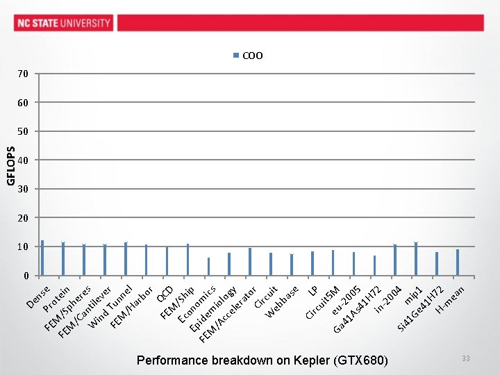
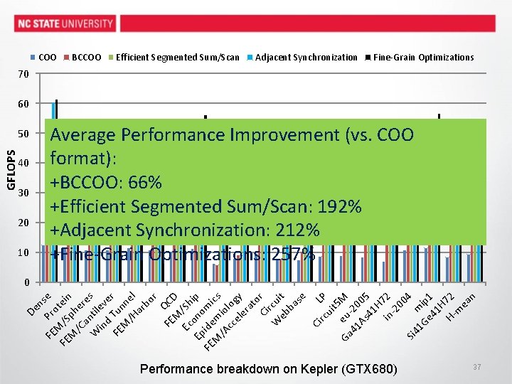
FE n Pr se M o FE /S tein M ph /C er a e W ntil s in ev d e FE Tun r M n /H el ar bo r Q FE CD M Ec /Sh Ep ono ip FE ide mi M m cs /A io cc log el y er at o Ci r W rcui eb t ba se Ci rc LP ui t 5 e Ga u M 41 -20 As 05 41 H 7 in 2 -2 00 4 Si 4 m 1 G ip e 4 1 1 H H- 72 m ea n De GFLOPS COO 70 60 50 40 30 20 10 0 Performance breakdown on Kepler (GTX 680) 33

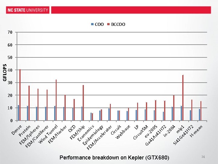
FE n Pr se M o FE /S tein M ph /C er a e W ntil s in ev d e FE Tun r M n /H el ar bo r Q FE CD M Ec /Sh Ep ono ip FE ide mi M m cs /A io cc log el y er at o Ci r W rcui eb t ba se Ci rc LP ui t 5 e Ga u M 41 -20 As 05 41 H 7 in 2 -2 00 4 Si 4 m 1 G ip e 4 1 1 H H- 72 m ea n De GFLOPS COO BCCOO 70 60 50 40 30 20 10 0 Performance breakdown on Kepler (GTX 680) 34

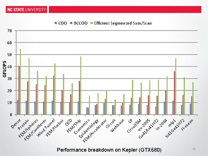
FE n Pr se M o FE /S tein M ph /C er a e W ntil s in ev d e FE Tun r M n /H el ar bo r Q FE CD M Ec /Sh Ep ono ip FE ide mi M m cs /A io cc log el y er at o Ci r W rcui eb t ba se Ci rc LP ui t 5 e Ga u M 41 -20 As 05 41 H 7 in 2 -2 00 4 Si 4 m 1 G ip e 4 1 1 H H- 72 m ea n De GFLOPS COO BCCOO Efficient Segmented Sum/Scan 70 60 50 40 30 20 10 0 Performance breakdown on Kepler (GTX 680) 35

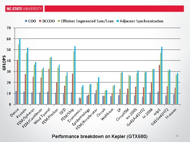
FE n Pr se M o FE /S tein M ph /C er a e W ntil s in ev d e FE Tun r M n /H el ar bo r Q FE CD M Ec /Sh Ep ono ip FE ide mi M m cs /A io cc log el y er at o Ci r W rcui eb t ba se Ci rc LP ui t 5 e Ga u M 41 -20 As 05 41 H 7 in 2 -2 00 4 Si 4 m 1 G ip e 4 1 1 H H- 72 m ea n De GFLOPS COO BCCOO Efficient Segmented Sum/Scan Adjacent Synchronization 70 60 50 40 30 20 10 0 Performance breakdown on Kepler (GTX 680) 36

COO BCCOO Efficient Segmented Sum/Scan Adjacent Synchronization Fine-Grain Optimizations 70 60 GFLOPS 50 40 30 20 10 Average Performance Improvement (vs. COO format): +BCCOO: 66% +Efficient Segmented Sum/Scan: 192% +Adjacent Synchronization: 212% +Fine-Grain Optimizations: 257% De ns FE Pro e M FE /S tein M ph /C er a e W ntil s in ev d e FE Tun r M n /H el ar bo r Q FE CD M Ec /Sh Ep ono ip FE ide mi M m cs /A io cc log el y er at o Ci r W rcui eb t ba se Ci rc LP ui t 5 e Ga u M 41 -20 As 05 41 H 7 in 2 -2 00 4 Si 4 m 1 G ip e 4 1 1 H H- 72 m ea n 0 Performance breakdown on Kepler (GTX 680) 37

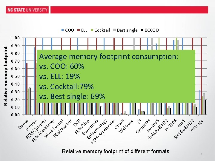
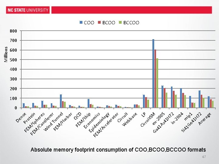
De ns P FE r e M o FE /S tein M ph /C er a e W ntil s in ev d e FE Tun r M n /H el ar bo r Q FE C M D Ec /Sh Ep ono ip FE ide mi M m cs /A io cc log el y er at o Ci r W rcui eb t ba se Ci rc LP ui t 5 Ga eu M 41 -20 As 05 41 H in 72 -2 00 4 Si 4 m 1 G ip e 4 1 1 H Av 72 er ag e Relative memory footprint COO 0. 80 0. 70 0. 60 0. 50 0. 40 0. 30 0. 20 ELL Cocktail Best single BCCOO 1. 00 0. 90 Average memory footprint consumption: vs. COO: 60% vs. ELL: 19% vs. Cocktail: 79% vs. Best single: 69% 0. 10 0. 00 Relative memory footprint of different formats 38

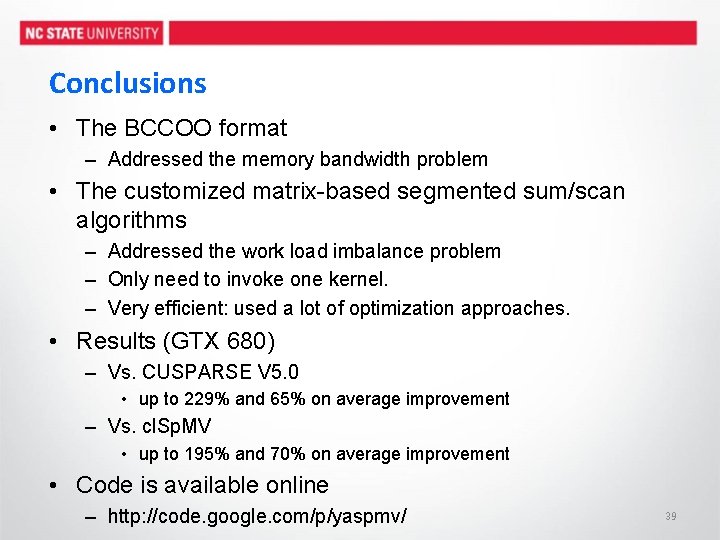
Conclusions • The BCCOO format – Addressed the memory bandwidth problem • The customized matrix-based segmented sum/scan algorithms – Addressed the work load imbalance problem – Only need to invoke one kernel. – Very efficient: used a lot of optimization approaches. • Results (GTX 680) – Vs. CUSPARSE V 5. 0 • up to 229% and 65% on average improvement – Vs. cl. Sp. MV • up to 195% and 70% on average improvement • Code is available online – http: //code. google. com/p/yaspmv/ 39

Thanks & Question? 40

COO format 41

COO format 3 0 2 42

COO format 36 00 26 43

Step 2 Segmented sum/scan • 3) Accumulating partial sums across workgroups Generate Partial Sums P 0 Step 3 Generate Partial Sums P 1 Step 3 Generate Partial Sums P 2 P 3 Step 3 Using Adjacent Synchronization 44

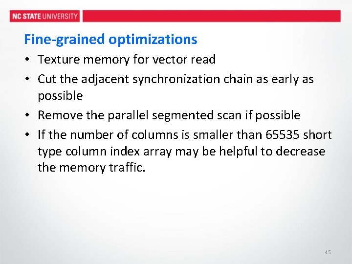
Fine-grained optimizations • Texture memory for vector read • Cut the adjacent synchronization chain as early as possible • Remove the parallel segmented scan if possible • If the number of columns is smaller than 65535 short type column index array may be helpful to decrease the memory traffic. 45

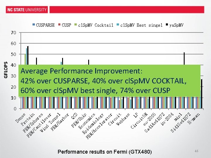
CUSPARSE CUSP cl. Sp. MV Cocktail cl. Sp. MV Best singel ya. Sp. MV 70 60 40 30 20 10 Average Performance Improvement: 42% over CUSPARSE, 40% over cl. Sp. MV COCKTAIL, 60% over cl. Sp. MV best single, 74% over CUSP 0 De ns P r FE o e FE M/ te M/ Sp in Ca he nt re Wi il s nd ev er FE Tun M/ ne Ha l rb or FE QC M D Ec /Sh E on ip FE pid om M/ em ic Ac io s ce lo le gy ra Ci tor rc We uit bb as e Ci rc LP ui t 5 e u Ga - M 41 20 As 05 41 in H 72 -2 00 4 Si m 41 i Ge p 1 41 H H- 72 me an GFLOPS 50 Performance results on Fermi (GTX 480) 46

ns P FE ro e M FE /S tein M ph /C er a e W ntile s in d ver FE Tun M ne /H l ar bo r FE QCD M Ec /Sh Ep ono ip FE ide mic M m s /A iol cc og el y er at o Ci r r W cui eb t ba se Ci rc LP ui t 5 Ga eu M 41 -20 As 05 41 H 7 in 2 -2 00 4 Si 4 m 1 G ip e 4 1 1 H Av 72 er ag e De Millions COO BCCOO 800 700 600 500 400 300 200 100 0 Absolute memory footprint consumption of COO, BCCOO formats 47