Using ranking and DCE data to value health

Using ranking and DCE data to value health states on the QALY scale using conventional and Bayesian methods Theresa Cain

AQl-5 D Data • Used ‘warm’ DCE data set • 168 individuals value 8 pairs of health states • A sample of 32 pairs of AQL-5 D health states valued

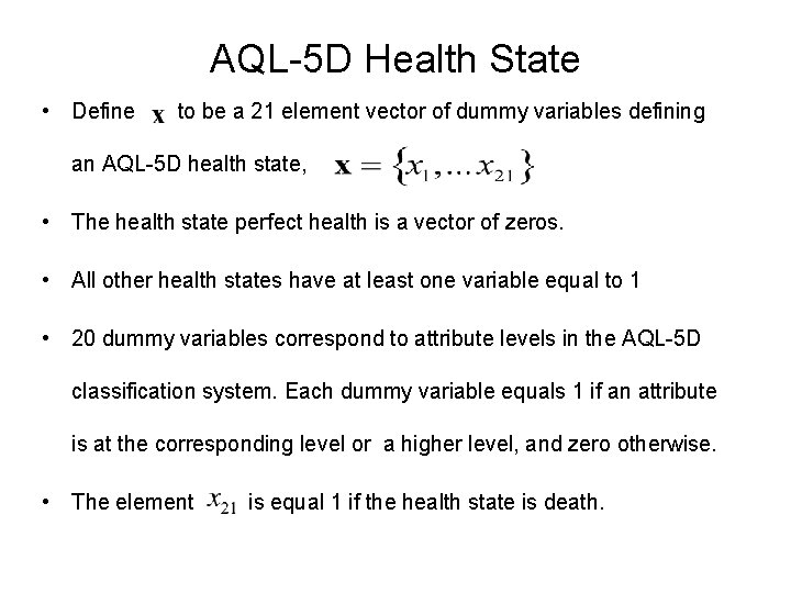
AQL-5 D Health State • Define to be a 21 element vector of dummy variables defining an AQL-5 D health state, • The health state perfect health is a vector of zeros. • All other health states have at least one variable equal to 1 • 20 dummy variables correspond to attribute levels in the AQL-5 D classification system. Each dummy variable equals 1 if an attribute is at the corresponding level or a higher level, and zero otherwise. • The element is equal 1 if the health state is death.

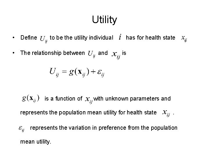
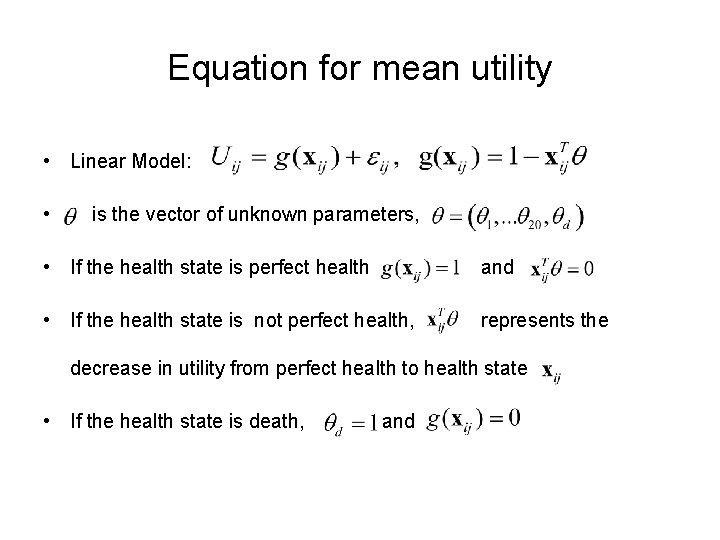
Utility • Define to be the utility individual • The relationship between is a function of and has for health state is with unknown parameters and represents the population mean utility for health state . represents the variation in preference from the population mean utility.

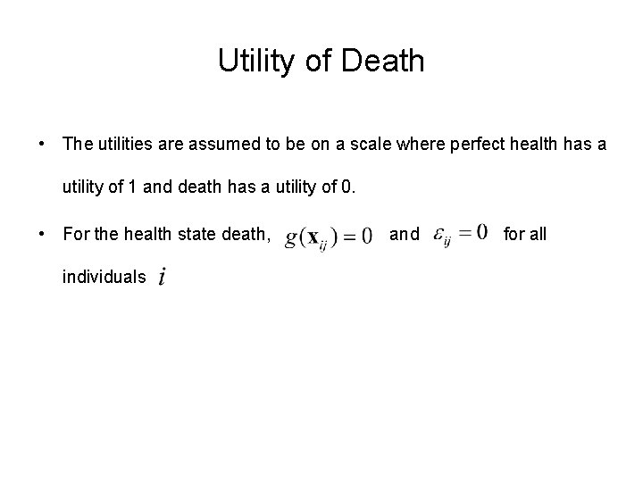
Utility of Death • The utilities are assumed to be on a scale where perfect health has a utility of 1 and death has a utility of 0. • For the health state death, individuals and for all

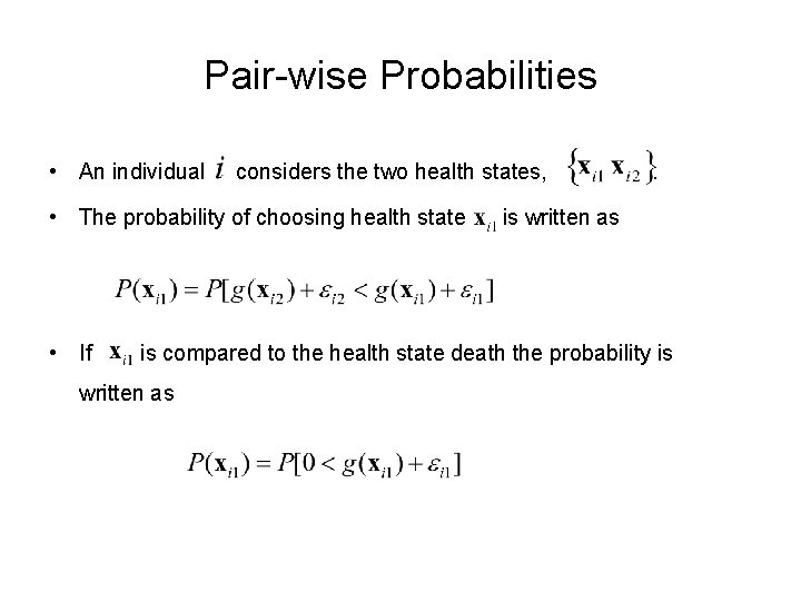
Pair-wise Probabilities • An individual considers the two health states, • The probability of choosing health state • If . is written as is compared to the health state death the probability is written as

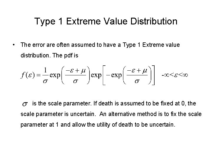
Type 1 Extreme Value Distribution • The error are often assumed to have a Type 1 Extreme value distribution. The pdf is is the scale parameter. If death is assumed to be fixed at 0, the scale parameter is uncertain. An alternative method is to fix the scale parameter at 1 and allow the utility of death to be uncertain.

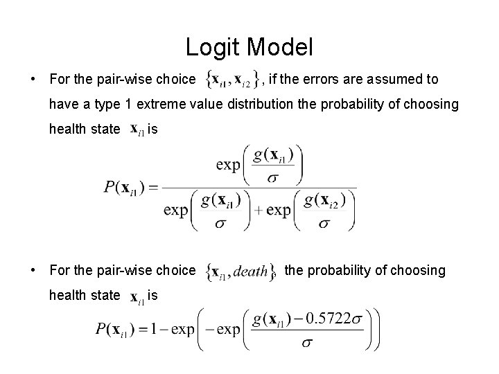
Logit Model • For the pair-wise choice , if the errors are assumed to have a type 1 extreme value distribution the probability of choosing health state is • For the pair-wise choice health state is , the probability of choosing

Equation for mean utility • Linear Model: • is the vector of unknown parameters, • If the health state is perfect health and • If the health state is not perfect health, represents the decrease in utility from perfect health to health state • If the health state is death, and

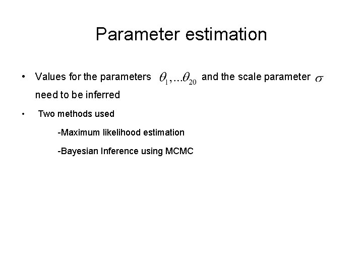
Parameter estimation • Values for the parameters need to be inferred • Two methods used -Maximum likelihood estimation -Bayesian Inference using MCMC and the scale parameter

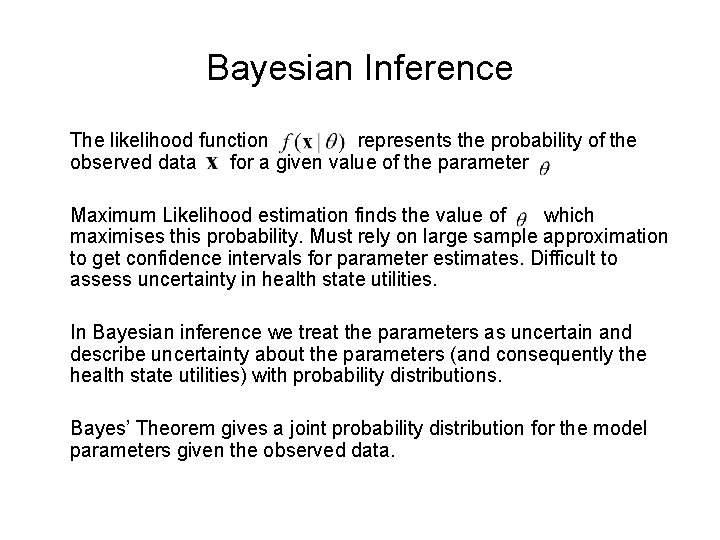
Bayesian Inference The likelihood function represents the probability of the observed data for a given value of the parameter Maximum Likelihood estimation finds the value of which maximises this probability. Must rely on large sample approximation to get confidence intervals for parameter estimates. Difficult to assess uncertainty in health state utilities. In Bayesian inference we treat the parameters as uncertain and describe uncertainty about the parameters (and consequently the health state utilities) with probability distributions. Bayes’ Theorem gives a joint probability distribution for the model parameters given the observed data.

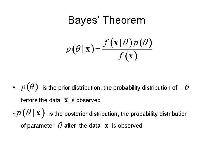
Bayes’ Theorem • is the prior distribution, the probability distribution of before the data • is observed is the posterior distribution, the probability distribution of parameter after the data is observed

Posterior Distribution • The posterior distribution represents the uncertainty about the parameters given the observed data • Important to understand uncertainty in parameters and therefore utilities • The posterior distribution cannot be derived analytically. A simulation method must be used to sample from the distribution. The sample will converge to the posterior distribution.

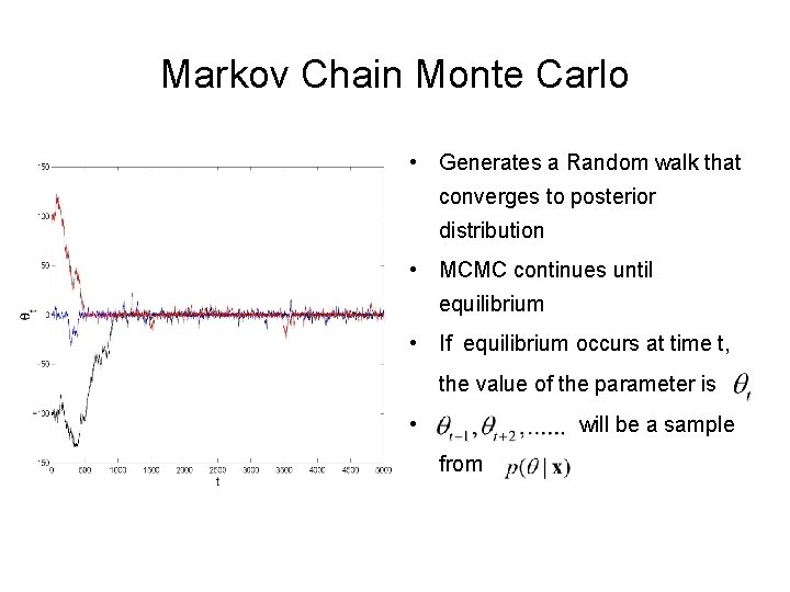
Markov Chain Monte Carlo • Generates a Random walk that converges to posterior distribution • MCMC continues until equilibrium • If equilibrium occurs at time t, the value of the parameter is • will be a sample from

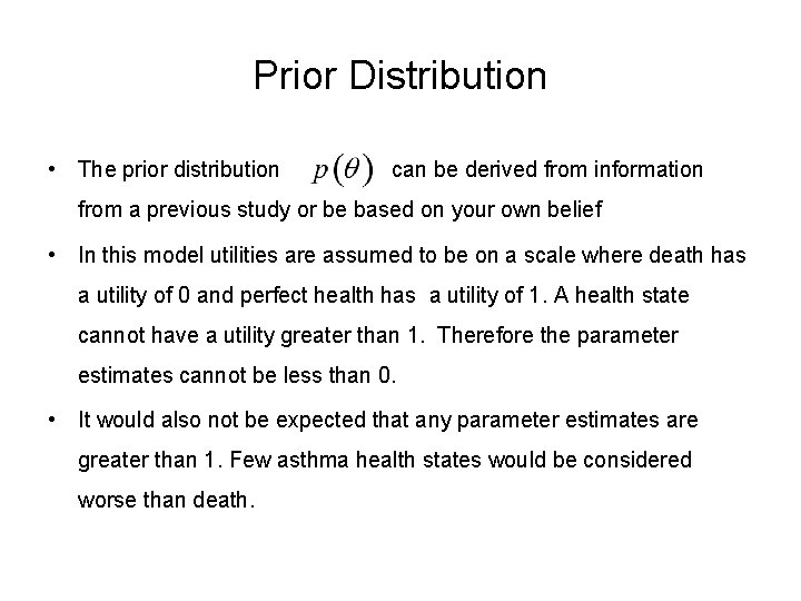
Prior Distribution • The prior distribution can be derived from information from a previous study or be based on your own belief • In this model utilities are assumed to be on a scale where death has a utility of 0 and perfect health has a utility of 1. A health state cannot have a utility greater than 1. Therefore the parameter estimates cannot be less than 0. • It would also not be expected that any parameter estimates are greater than 1. Few asthma health states would be considered worse than death.

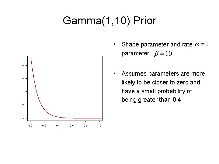
Gamma(1, 10) Prior • Shape parameter and rate parameter • Assumes parameters are more likely to be closer to zero and have a small probability of being greater than 0. 4

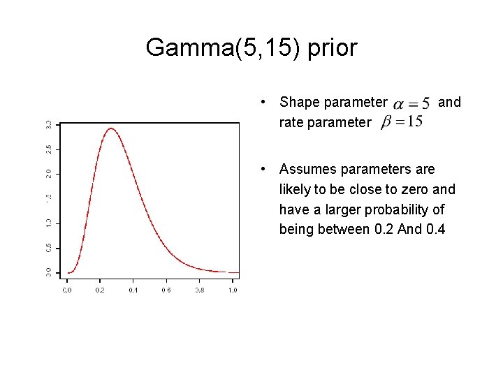
Gamma(5, 15) prior • Shape parameter rate parameter and • Assumes parameters are likely to be close to zero and have a larger probability of being between 0. 2 And 0. 4

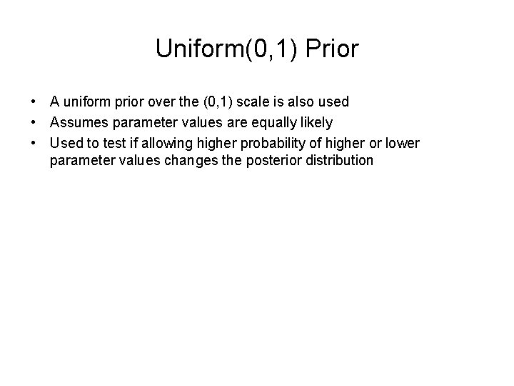
Uniform(0, 1) Prior • A uniform prior over the (0, 1) scale is also used • Assumes parameter values are equally likely • Used to test if allowing higher probability of higher or lower parameter values changes the posterior distribution

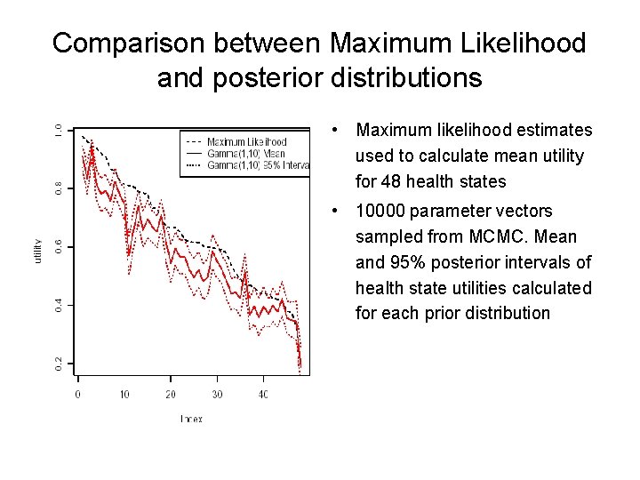
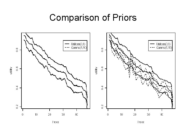
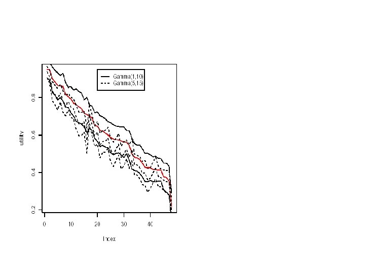
Comparison between Maximum Likelihood and posterior distributions • Maximum likelihood estimates used to calculate mean utility for 48 health states • 10000 parameter vectors sampled from MCMC. Mean and 95% posterior intervals of health state utilities calculated for each prior distribution

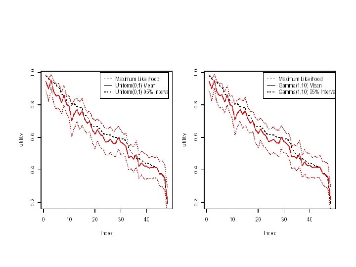
Comparison of Priors

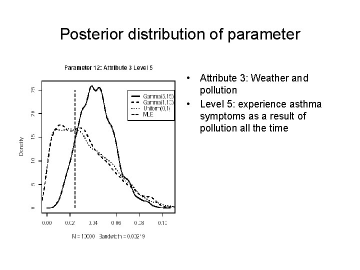
Posterior distribution of parameter • Attribute 3: Weather and pollution • Level 5: experience asthma symptoms as a result of pollution all the time

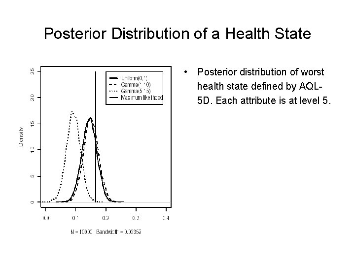
Posterior Distribution of a Health State • Posterior distribution of worst health state defined by AQL 5 D. Each attribute is at level 5.

Conclusion • Posterior distributions similar when Gamma(1, 10) and Uniform(0, 1) prior • If the prior distribution does not favour larger values the posterior distribution is robust to the prior • Posterior intervals might not be precise enough to use in an economic evaluation.