University of Warwick Department of Sociology 201213 SO

University of Warwick, Department of Sociology, 2012/13 SO 201: SSAASS (Surveys and Statistics) (Richard Lampard) Analysing Means I: (Extending) Analysis of Variance (Week 14)

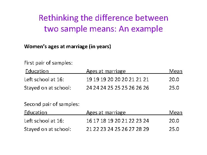
Rethinking the difference between two sample means: An example Women’s ages at marriage (in years) First pair of samples: Education Left school at 16: Stayed on at school: Ages at marriage 19 19 19 20 20 20 21 21 21 24 24 24 25 25 25 26 26 26 Mean 20. 0 25. 0 Second pair of samples: Education Left school at 16: Stayed on at school: Ages at marriage 16 17 18 19 20 21 22 23 24 25 26 27 28 29 Mean 20. 0 25. 0

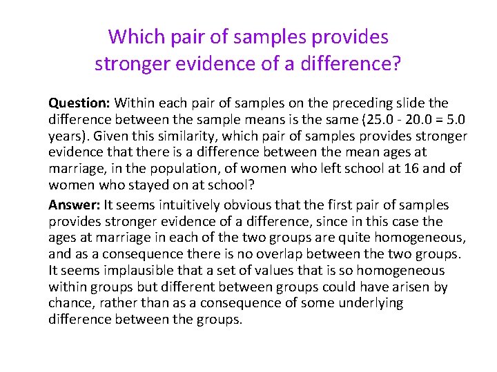
Which pair of samples provides stronger evidence of a difference? Question: Within each pair of samples on the preceding slide the difference between the sample means is the same (25. 0 - 20. 0 = 5. 0 years). Given this similarity, which pair of samples provides stronger evidence that there is a difference between the mean ages at marriage, in the population, of women who left school at 16 and of women who stayed on at school? Answer: It seems intuitively obvious that the first pair of samples provides stronger evidence of a difference, since in this case the ages at marriage in each of the two groups are quite homogeneous, and as a consequence there is no overlap between the two groups. It seems implausible that a set of values that is so homogeneous within groups but different between groups could have arisen by chance, rather than as a consequence of some underlying difference between the groups.

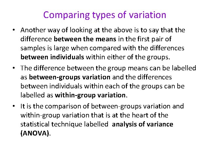
Comparing types of variation • Another way of looking at the above is to say that the difference between the means in the first pair of samples is large when compared with the differences between individuals within either of the groups. • The difference between the group means can be labelled as between-groups variation and the differences between individuals within each of the groups can be labelled as within-group variation. • It is the comparison of between-groups variation and within-group variation that is at the heart of the statistical technique labelled analysis of variance (ANOVA).

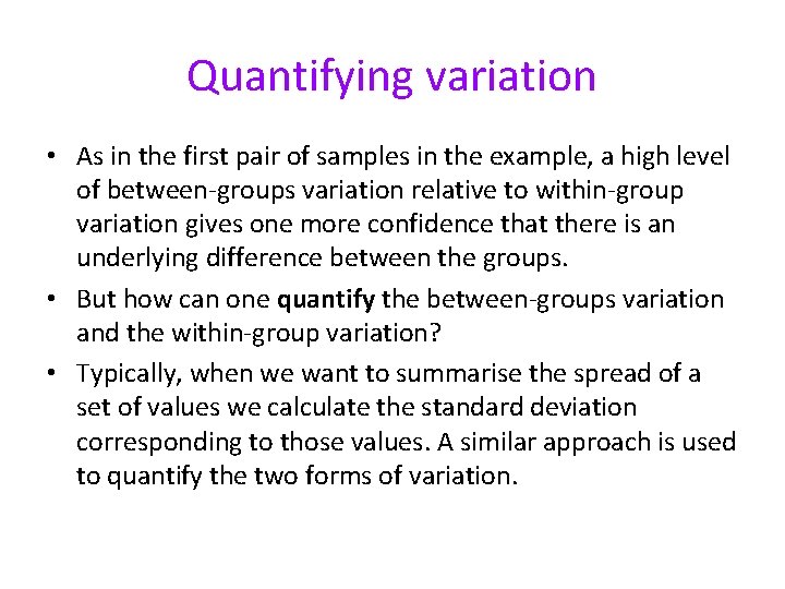
Quantifying variation • As in the first pair of samples in the example, a high level of between-groups variation relative to within-group variation gives one more confidence that there is an underlying difference between the groups. • But how can one quantify the between-groups variation and the within-group variation? • Typically, when we want to summarise the spread of a set of values we calculate the standard deviation corresponding to those values. A similar approach is used to quantify the two forms of variation.

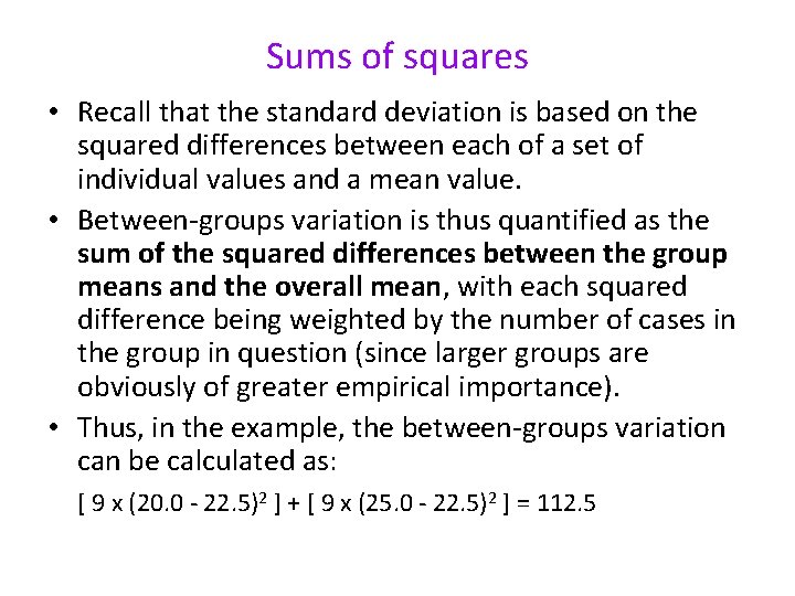
Sums of squares • Recall that the standard deviation is based on the squared differences between each of a set of individual values and a mean value. • Between-groups variation is thus quantified as the sum of the squared differences between the group means and the overall mean, with each squared difference being weighted by the number of cases in the group in question (since larger groups are obviously of greater empirical importance). • Thus, in the example, the between-groups variation can be calculated as: [ 9 x (20. 0 - 22. 5)2 ] + [ 9 x (25. 0 - 22. 5)2 ] = 112. 5

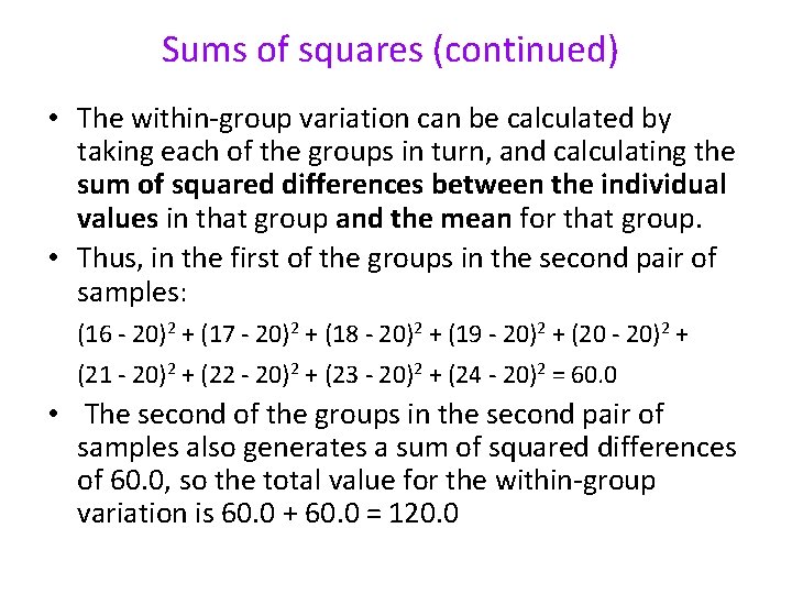
Sums of squares (continued) • The within-group variation can be calculated by taking each of the groups in turn, and calculating the sum of squared differences between the individual values in that group and the mean for that group. • Thus, in the first of the groups in the second pair of samples: (16 - 20)2 + (17 - 20)2 + (18 - 20)2 + (19 - 20)2 + (20 - 20)2 + (21 - 20)2 + (22 - 20)2 + (23 - 20)2 + (24 - 20)2 = 60. 0 • The second of the groups in the second pair of samples also generates a sum of squared differences of 60. 0, so the total value for the within-group variation is 60. 0 + 60. 0 = 120. 0

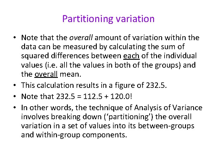
Partitioning variation • Note that the overall amount of variation within the data can be measured by calculating the sum of squared differences between each of the individual values (i. e. all the values in both of the groups) and the overall mean. • This calculation results in a figure of 232. 5. • Note that 232. 5 = 112. 5 + 120. 0! • In other words, the technique of Analysis of Variance involves breaking down (‘partitioning’) the overall variation in a set of values into its between-groups and within-group components.

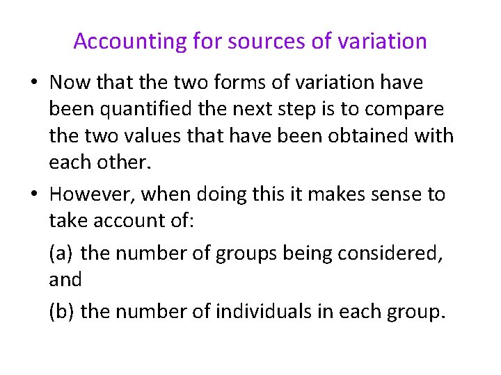
Accounting for sources of variation • Now that the two forms of variation have been quantified the next step is to compare the two values that have been obtained with each other. • However, when doing this it makes sense to take account of: (a) the number of groups being considered, and (b) the number of individuals in each group.

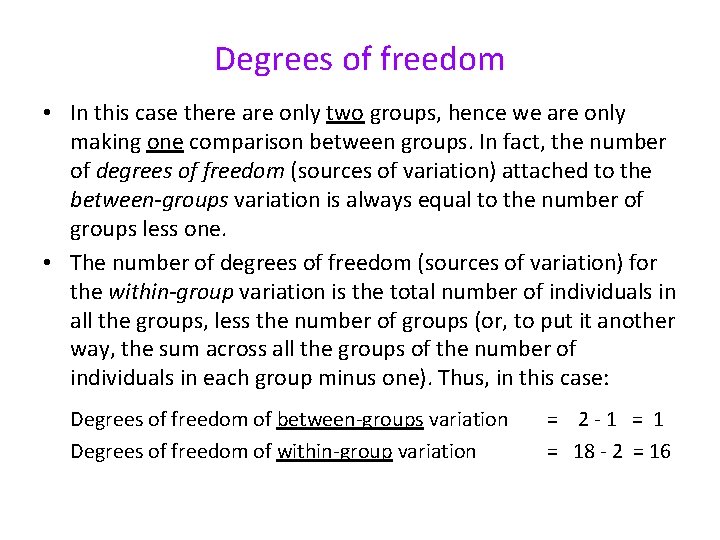
Degrees of freedom • In this case there are only two groups, hence we are only making one comparison between groups. In fact, the number of degrees of freedom (sources of variation) attached to the between-groups variation is always equal to the number of groups less one. • The number of degrees of freedom (sources of variation) for the within-group variation is the total number of individuals in all the groups, less the number of groups (or, to put it another way, the sum across all the groups of the number of individuals in each group minus one). Thus, in this case: Degrees of freedom of between-groups variation Degrees of freedom of within-group variation = 2 -1 = 18 - 2 = 16

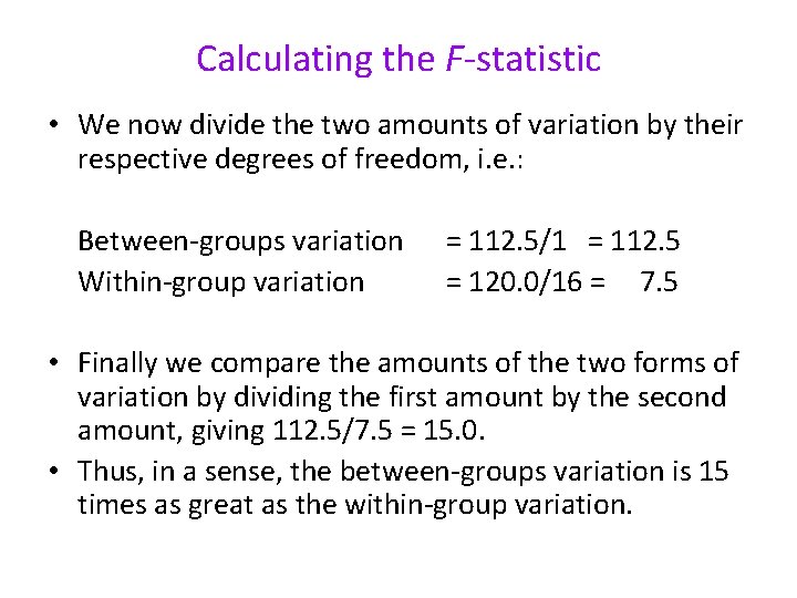
Calculating the F-statistic • We now divide the two amounts of variation by their respective degrees of freedom, i. e. : Between-groups variation Within-group variation = 112. 5/1 = 112. 5 = 120. 0/16 = 7. 5 • Finally we compare the amounts of the two forms of variation by dividing the first amount by the second amount, giving 112. 5/7. 5 = 15. 0. • Thus, in a sense, the between-groups variation is 15 times as great as the within-group variation.

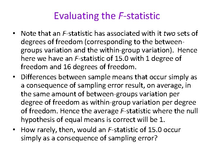
Evaluating the F-statistic • Note that an F-statistic has associated with it two sets of degrees of freedom (corresponding to the betweengroups variation and the within-group variation). Hence here we have an F-statistic of 15. 0 with 1 degree of freedom and 16 degrees of freedom. • Differences between sample means that occur simply as a consequence of sampling error result, on average, in the same amount of between-groups variation per degree of freedom as within-group variation per degree of freedom. Hence the average F-statistic where the null hypothesis of equal means is correct will be 1. • How rarely, then, would an F-statistic of 15. 0 occur simply as a consequence of sampling error?

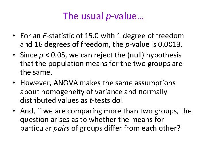
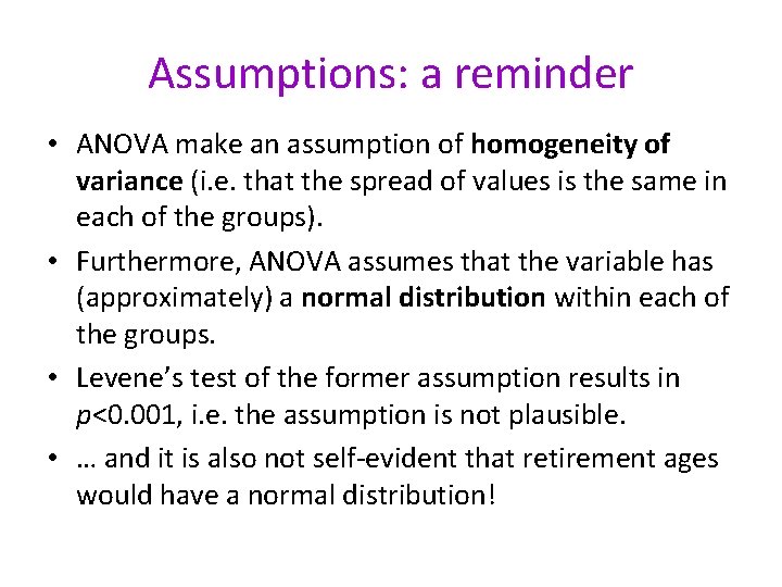
The usual p-value… • For an F-statistic of 15. 0 with 1 degree of freedom and 16 degrees of freedom, the p-value is 0. 0013. • Since p < 0. 05, we can reject the (null) hypothesis that the population means for the two groups are the same. • However, ANOVA makes the same assumptions about homogeneity of variance and normally distributed values as t-tests do! • And, if we are comparing more than two groups, the question arises as to whether the means for particular pairs of groups differ from each other?

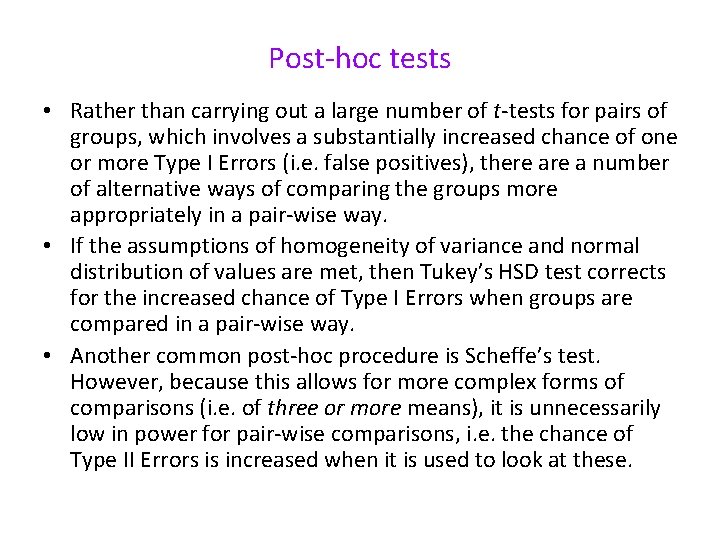
Post-hoc tests • Rather than carrying out a large number of t-tests for pairs of groups, which involves a substantially increased chance of one or more Type I Errors (i. e. false positives), there a number of alternative ways of comparing the groups more appropriately in a pair-wise way. • If the assumptions of homogeneity of variance and normal distribution of values are met, then Tukey’s HSD test corrects for the increased chance of Type I Errors when groups are compared in a pair-wise way. • Another common post-hoc procedure is Scheffe’s test. However, because this allows for more complex forms of comparisons (i. e. of three or more means), it is unnecessarily low in power for pair-wise comparisons, i. e. the chance of Type II Errors is increased when it is used to look at these.

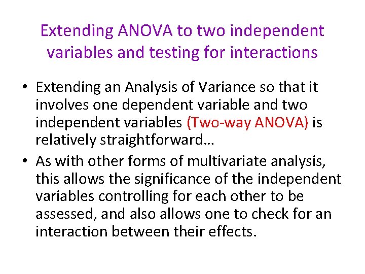
Extending ANOVA to two independent variables and testing for interactions • Extending an Analysis of Variance so that it involves one dependent variable and two independent variables (Two-way ANOVA) is relatively straightforward… • As with other forms of multivariate analysis, this allows the significance of the independent variables controlling for each other to be assessed, and also allows one to check for an interaction between their effects.

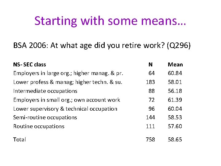
Starting with some means… BSA 2006: At what age did you retire work? (Q 296) NS- SEC class Employers in large org. ; higher manag. & pr. Lower profess & manag; higher techn. & su. Intermediate occupations Employers in small org. ; own account work Lower supervisory & technical occupation Semi-routine occupations Routine occupations N 64 183 88 72 96 144 111 Mean 60. 84 58. 01 56. 18 61. 39 60. 04 58. 53 57. 60 Total 758 58. 65

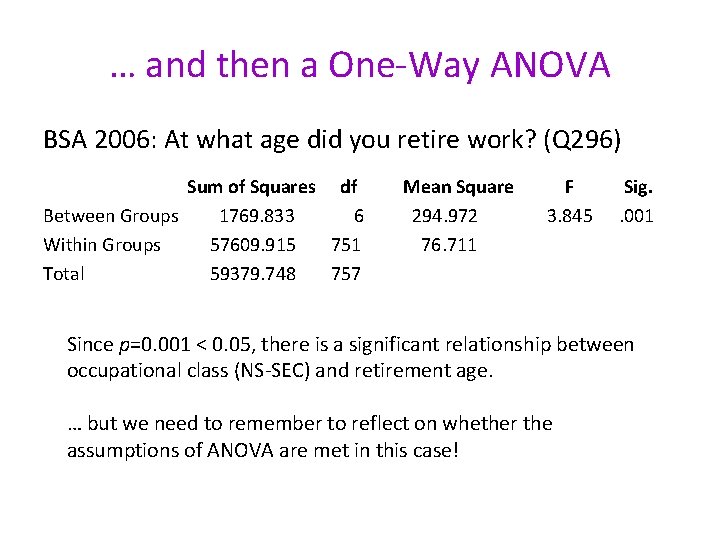
… and then a One-Way ANOVA BSA 2006: At what age did you retire work? (Q 296) Sum of Squares df Between Groups 1769. 833 6 Within Groups 57609. 915 751 Total 59379. 748 757 Mean Square 294. 972 76. 711 F 3. 845 Sig. . 001 Since p=0. 001 < 0. 05, there is a significant relationship between occupational class (NS-SEC) and retirement age. … but we need to remember to reflect on whether the assumptions of ANOVA are met in this case!

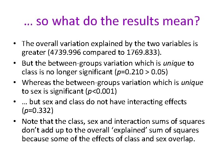
Assumptions: a reminder • ANOVA make an assumption of homogeneity of variance (i. e. that the spread of values is the same in each of the groups). • Furthermore, ANOVA assumes that the variable has (approximately) a normal distribution within each of the groups. • Levene’s test of the former assumption results in p<0. 001, i. e. the assumption is not plausible. • … and it is also not self-evident that retirement ages would have a normal distribution!

Nevertheless… • We might ask ourselves the question whether some of the class difference in retirement ages reflects gender. • And hence there is a motivation to carry out a Two-way ANOVA to look at the effects of class and gender simultaneously.

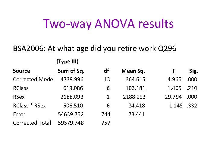
Two-way ANOVA results BSA 2006: At what age did you retire work Q 296 (Type III) Source Corrected Model RClass RSex RClass * RSex Error Corrected Total Sum of Sq. 4739. 996 619. 086 2188. 093 506. 510 54639. 752 59379. 748 df 13 6 1 6 744 757 Mean Sq. 364. 615 103. 181 2188. 093 84. 418 73. 441 F 4. 965 1. 405 29. 794 1. 149 Sig. . 000. 210. 000. 332

… so what do the results mean? • The overall variation explained by the two variables is greater (4739. 996 compared to 1769. 833). • But the between-groups variation which is unique to class is no longer significant (p=0. 210 > 0. 05) • Whereas the between-groups variation which is unique to sex is significant (p<0. 001) • … but sex and class do not have interacting effects (p=0. 332) • Note that the class, sex and interaction sums of squares don’t add up to the overall ‘explained’ sum of squares because some of the effects of class and sex overlap.

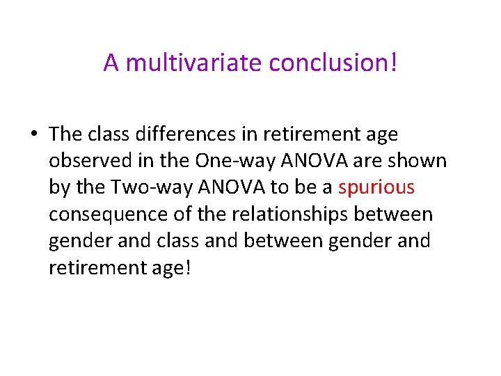
A multivariate conclusion! • The class differences in retirement age observed in the One-way ANOVA are shown by the Two-way ANOVA to be a spurious consequence of the relationships between gender and class and between gender and retirement age!

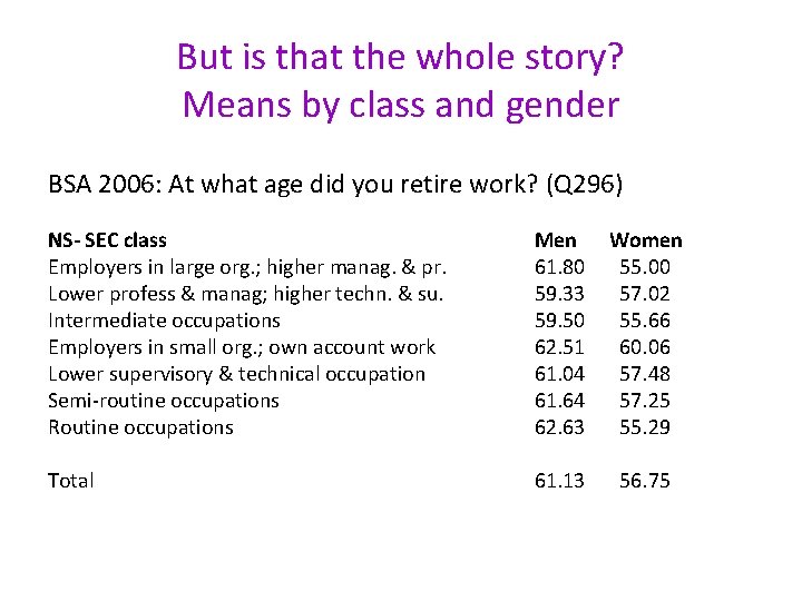
But is that the whole story? Means by class and gender BSA 2006: At what age did you retire work? (Q 296) NS- SEC class Employers in large org. ; higher manag. & pr. Lower profess & manag; higher techn. & su. Intermediate occupations Employers in small org. ; own account work Lower supervisory & technical occupation Semi-routine occupations Routine occupations Men 61. 80 59. 33 59. 50 62. 51 61. 04 61. 64 62. 63 Women 55. 00 57. 02 55. 66 60. 06 57. 48 57. 25 55. 29 Total 61. 13 56. 75

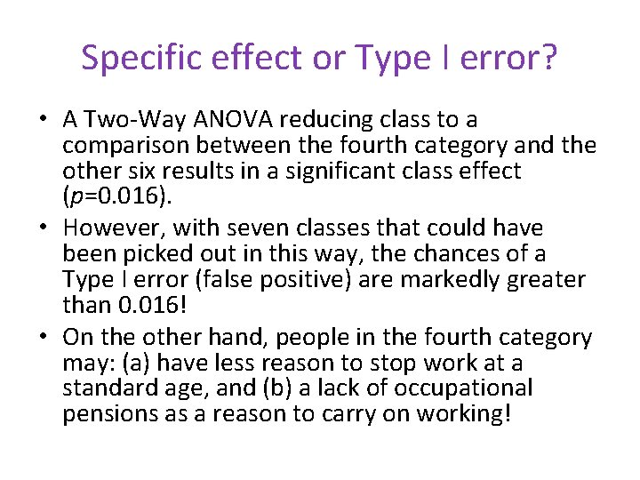
Specific effect or Type I error? • A Two-Way ANOVA reducing class to a comparison between the fourth category and the other six results in a significant class effect (p=0. 016). • However, with seven classes that could have been picked out in this way, the chances of a Type I error (false positive) are markedly greater than 0. 016! • On the other hand, people in the fourth category may: (a) have less reason to stop work at a standard age, and (b) a lack of occupational pensions as a reason to carry on working!

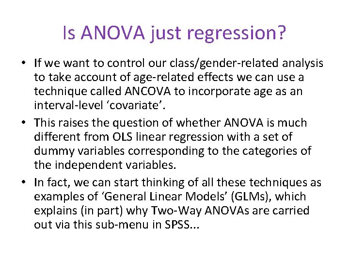
Is ANOVA just regression? • If we want to control our class/gender-related analysis to take account of age-related effects we can use a technique called ANCOVA to incorporate age as an interval-level ‘covariate’. • This raises the question of whether ANOVA is much different from OLS linear regression with a set of dummy variables corresponding to the categories of the independent variables. • In fact, we can start thinking of all these techniques as examples of ‘General Linear Models’ (GLMs), which explains (in part) why Two-Way ANOVAs are carried out via this sub-menu in SPSS. . .