University of Warwick Department of Sociology 201213 SO

University of Warwick, Department of Sociology, 2012/13 SO 201: SSAASS (Surveys and Statistics) (Richard Lampard) Logistic Regression II/ (Hierarchical) Log-Linear Models I

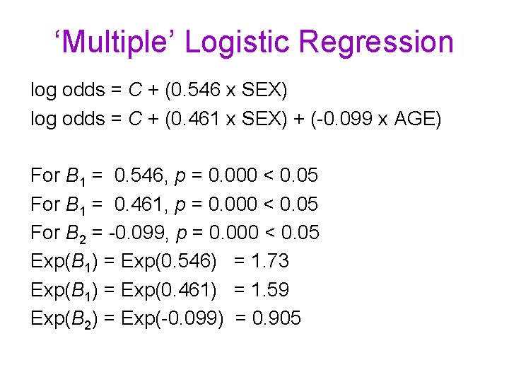
‘Multiple’ Logistic Regression log odds = C + (0. 546 x SEX) log odds = C + (0. 461 x SEX) + (-0. 099 x AGE) For B 1 = 0. 546, p = 0. 000 < 0. 05 For B 1 = 0. 461, p = 0. 000 < 0. 05 For B 2 = -0. 099, p = 0. 000 < 0. 05 Exp(B 1) = Exp(0. 546) = 1. 73 Exp(B 1) = Exp(0. 461) = 1. 59 Exp(B 2) = Exp(-0. 099) = 0. 905

• The odds ratio comparing men with women and controlling for age is 1. 59, less than the original value of 1. 73. • Thus some, but not all, of the gender difference in having (any) teeth can be accounted for in terms of age. • The odds ratio of 0. 905 for age indicates that the odds of having any teeth decrease by more than 9% for each extra year of age (since 1 - 0. 905 = 0. 095 = 9. 5%). • In other words the odds of having no teeth increase by over 10% for each extra year of age! (since 1/0. 905 = 1. 105).

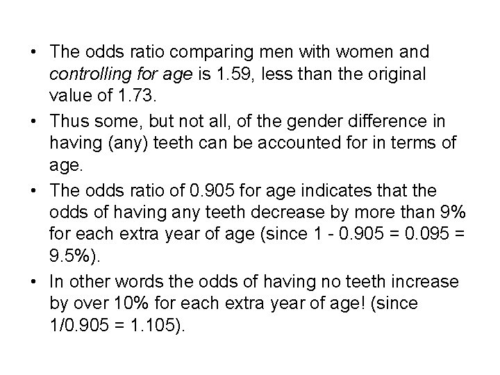
Adding Father’s Class Sex Age Father’s Class ‘None’ vs I/II vs III NM vs III M vs Constant IV/V B p. 471. 000 -. 097. 000. 504. 007 1. 374. 000 1. 432. 000. 463. 008 6. 132 Exp(B) 1. 602. 908 1. 656 3. 950 4. 187 1. 588

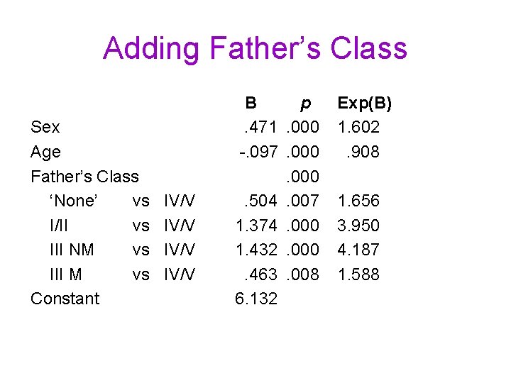
Adding Own Class B Father’s class ‘None’ vs I/II vs III NM vs III M vs Own class ‘None’ vs I/II vs III NM vs III M vs Constant IV/V . 342. 957. 974. 315 IV/V . 591 1. 474 1. 189. 416 5. 736 p. 002. 075. 000. 019. 079. 000. 052. 000. 003 Exp(B) 1. 407 2. 603 2. 648 1. 370 1. 805 4. 366 3. 284 1. 515

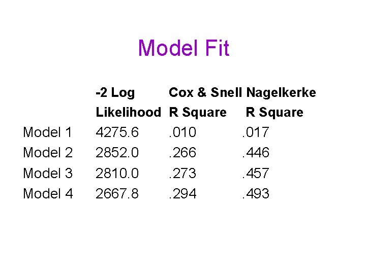
Model Fit -2 Log Cox & Snell Nagelkerke Likelihood R Square Model 1 Model 2 Model 3 Model 4 4275. 6 2852. 0 2810. 0 2667. 8 . 010. 266. 273. 294 . 017. 446. 457. 493

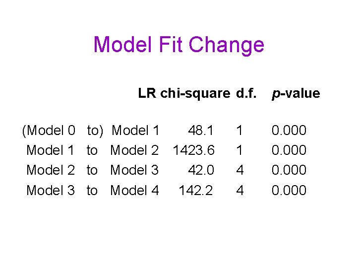
Model Fit Change LR chi-square d. f. (Model 0 Model 1 Model 2 Model 3 to) to to to Model 1 48. 1 Model 2 1423. 6 Model 3 42. 0 Model 4 142. 2 1 1 4 4 p-value 0. 000

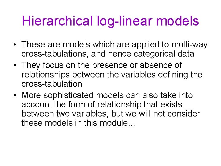
Hierarchical log-linear models • These are models which are applied to multi-way cross-tabulations, and hence categorical data • They focus on the presence or absence of relationships between the variables defining the cross-tabulation • More sophisticated models can also take into account the form of relationship that exists between two variables, but we will not consider these models in this module…

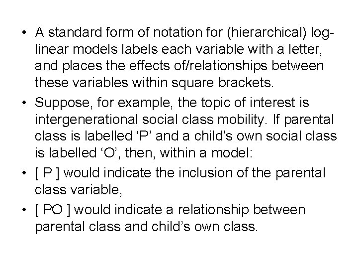
• A standard form of notation for (hierarchical) loglinear models labels each variable with a letter, and places the effects of/relationships between these variables within square brackets. • Suppose, for example, the topic of interest is intergenerational social class mobility. If parental class is labelled ‘P’ and a child’s own social class is labelled ‘O’, then, within a model: • [ P ] would indicate the inclusion of the parental class variable, • [ PO ] would indicate a relationship between parental class and child’s own class.

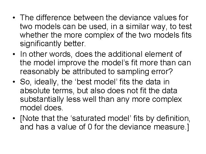
A bivariate analysis • Bivariate (hierarchical) log-linear models are of limited interest, but for illustrative purposes, there are two models of a two-way crosstabulation: • [ P ] [ O ], the ‘independence model’, which indicates that the two variables are unrelated. • [ PO ], an example of a ‘saturated model’, wherein all of the variables are related to each other simultaneously (i. e. in this simplest form of saturated model, the two variables are related).

‘Goodness (or ‘badness’)-of-fit • The model [ PO ] is consistent with any observed relationship in a cross-tabulation, and hence, by definition, fits the observed data perfectly. • It is therefore said to have a ‘goodness-offit’ value of 0. (Note that measures of ‘goodness-of-fit’ typically measure badness of fit!)

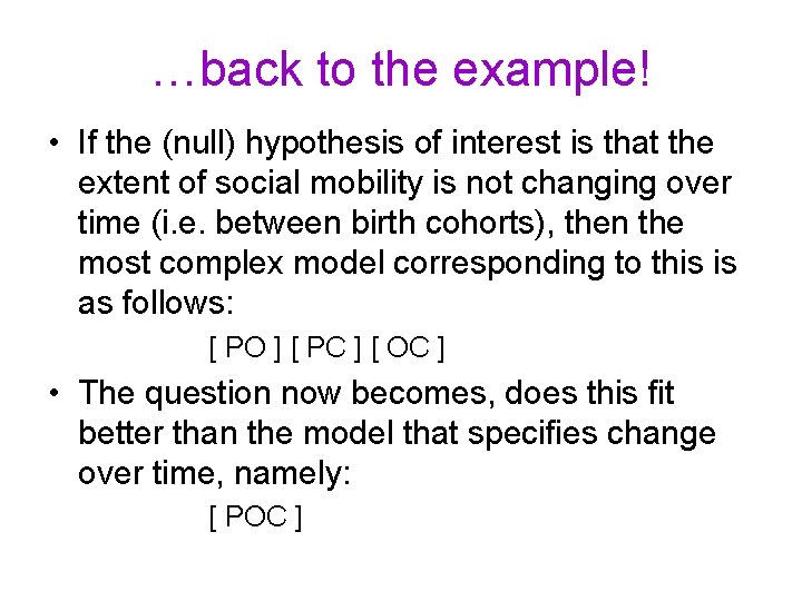
• Turning to the independence model, the ‘goodness-of-fit’ of [ P ] [ O ] can be viewed as equivalent to the chi-square statistic, as this summarises the evidence of a relationship, and hence the evidence that the (null) hypothesis of independence, i. e. the independence model, is incorrect. • In fact, it is the likelihood ratio chi-square statistic from SPSS output for a cross-tabulation which is relevant here. • A chi-square test is thus, in effect, a comparison (and choice) between two possible models of a two-way cross-tabulation.

A multivariate analysis • Suppose that one was interested in whether the extent of social mobility was changing over time (i. e. between birth cohorts). • Then we would need to include in any model a third variable, i. e. birth cohort, represented by ‘C’.

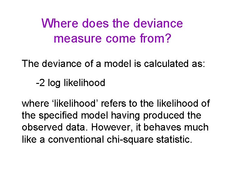
A wider choice of models… • For a three-way cross-tabulation, there a greater number of possible hierarchical models of the cross-tabulation: • The ‘independence model’ [ P ] [ O ] [ C ], • The ‘saturated model’ [ POC ], which indicates that the relationship between parental class and child’s own class varies according to birth cohort, and…

• …various other models in between these: • • [ PO ] [ C ] [ PC ] [ OC ] [ PO ] [ PC ] [ PO ] [ OC ] [ PC ] [ OC ] [ PO ] [ PC ] [ OC ]

How does one know which model is best? • Each model has a chi-square-like ‘goodness-offit’ measure, often referred to as the model’s deviance, which can be used to test whether the observed data is significantly different from what one would expect to have seen given that model. • In other words, to quantify how likely it is that the difference(s) between the observed data and the model’s predictions would have occurred simply as a consequence of sampling error.

• The difference between the deviance values for two models can be used, in a similar way, to test whether the more complex of the two models fits significantly better. • In other words, does the additional element of the model improve the model’s fit more than can reasonably be attributed to sampling error? • So, ideally, the ‘best model’ fits the data in absolute terms, but also does not fit the data substantially less well than any more complex model does. • [Note that the ‘saturated model’ fits by definition, and has a value of 0 for the deviance measure. ]

…back to the example! • If the (null) hypothesis of interest is that the extent of social mobility is not changing over time (i. e. between birth cohorts), then the most complex model corresponding to this is as follows: [ PO ] [ PC ] [ OC ] • The question now becomes, does this fit better than the model that specifies change over time, namely: [ POC ]

Where does the deviance measure come from? The deviance of a model is calculated as: -2 log likelihood where ‘likelihood’ refers to the likelihood of the specified model having produced the observed data. However, it behaves much like a conventional chi-square statistic.

What about degrees of freedom? • Each model deviance value has an associated number of degrees of freedom, relating to the various relationships between variables that are not included in the model. • Hence the ‘saturated model’ has zero degrees of freedom. • If the three variables, P, O and C had a, b and c categories, then the ‘independence model’ would have (a x b x c) – (a + b + c) + 2 degrees of freedom, e. g. 4 degrees of freedom if all the variables had two categories each.

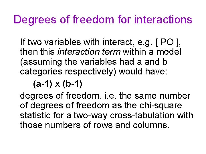
Degrees of freedom for interactions If two variables with interact, e. g. [ PO ], then this interaction term within a model (assuming the variables had a and b categories respectively) would have: (a-1) x (b-1) degrees of freedom, i. e. the same number of degrees of freedom as the chi-square statistic for a two-way cross-tabulation with those numbers of rows and columns.

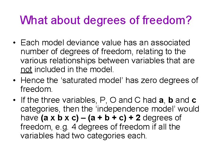
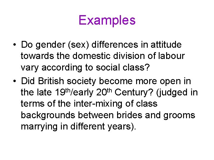
Examples • Do gender (sex) differences in attitude towards the domestic division of labour vary according to social class? • Did British society become more open in the late 19 th/early 20 th Century? (judged in terms of the inter-mixing of class backgrounds between brides and grooms marrying in different years).

The answer is ‘Yes’ in each case! • The model [CSA] fits significantly better than the model [CS][CA][SA] (p = 0. 046) • The model [BGY] fits significantly better than the model [BG][BY][GY] (p < 0. 001)