Umans Complexity Theory Lectures Worstcase vs Averagecase using

Umans Complexity Theory Lectures Worst-case vs. Average-case using Error-Correcting Codes: Transforming worst-case hardness into average-case hardness

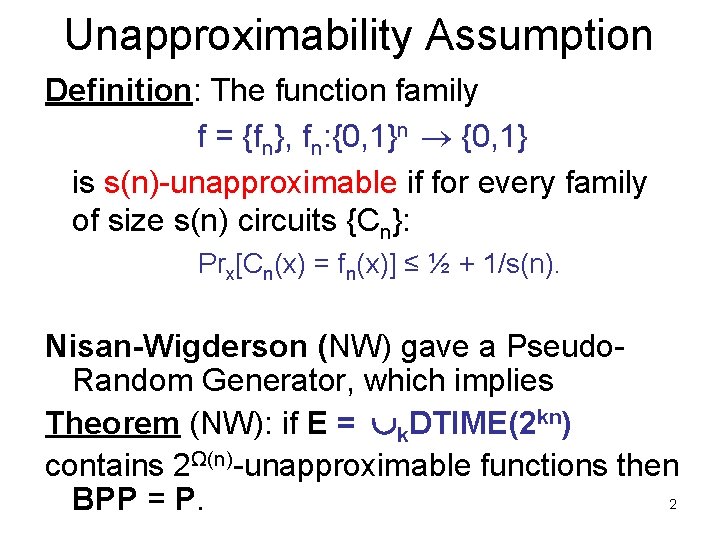
Unapproximability Assumption Definition: The function family f = {fn}, fn: {0, 1}n {0, 1} is s(n)-unapproximable if for every family of size s(n) circuits {Cn}: Prx[Cn(x) = fn(x)] ≤ ½ + 1/s(n). Nisan-Wigderson (NW) gave a Pseudo. Random Generator, which implies Theorem (NW): if E = k. DTIME(2 kn) contains 2Ω(n)-unapproximable functions then 2 BPP = P.

Unapproximability Assumption • How reasonable is unapproximability assumption? • Hope: obtain BPP = P from worst-case complexity assumption – try to fit into existing framework without new notion of “unapproximability” 3

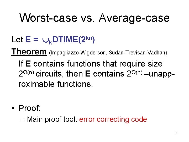
Worst-case vs. Average-case Let E = k. DTIME(2 kn) Theorem (Impagliazzo-Wigderson, Sudan-Trevisan-Vadhan) If E contains functions that require size 2Ω(n) circuits, then E contains 2Ω(n) –unapproximable functions. • Proof: – Main proof tool: error correcting code 4

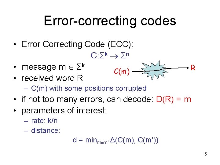
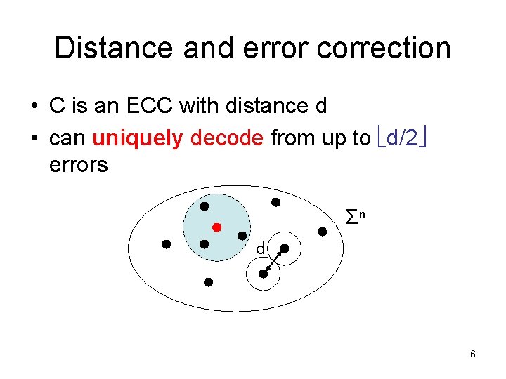
Error-correcting codes • Error Correcting Code (ECC): C: Σk Σn • message m Σk C(m) • received word R R – C(m) with some positions corrupted • if not too many errors, can decode: D(R) = m • parameters of interest: – rate: k/n – distance: d = minm m’ Δ(C(m), C(m’)) 5

Distance and error correction • C is an ECC with distance d • can uniquely decode from up to d/2 errors Σn d 6

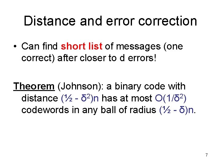
Distance and error correction • Can find short list of messages (one correct) after closer to d errors! Theorem (Johnson): a binary code with distance (½ - δ 2)n has at most O(1/δ 2) codewords in any ball of radius (½ - δ)n. 7

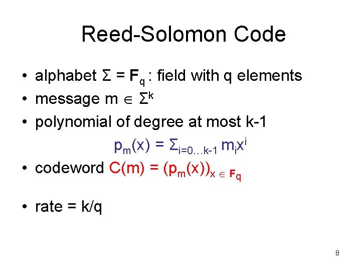
Reed-Solomon Code • alphabet Σ = Fq : field with q elements • message m Σk • polynomial of degree at most k-1 pm(x) = Σi=0…k-1 mixi • codeword C(m) = (pm(x))x Fq • rate = k/q 8

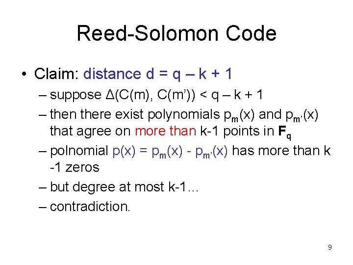
Reed-Solomon Code • Claim: distance d = q – k + 1 – suppose Δ(C(m), C(m’)) < q – k + 1 – then there exist polynomials pm(x) and pm’(x) that agree on more than k-1 points in Fq – polnomial p(x) = pm(x) - pm’(x) has more than k -1 zeros – but degree at most k-1… – contradiction. 9

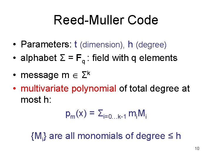
Reed-Muller Code • Parameters: t (dimension), h (degree) • alphabet Σ = Fq : field with q elements • message m Σk • multivariate polynomial of total degree at most h: pm(x) = Σi=0…k-1 mi. Mi {Mi} are all monomials of degree ≤ h 10

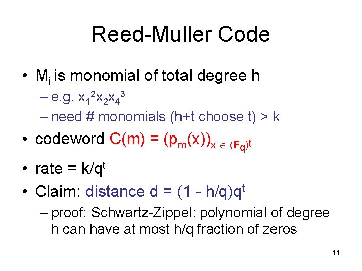
Reed-Muller Code • Mi is monomial of total degree h – e. g. x 12 x 2 x 43 – need # monomials (h+t choose t) > k • codeword C(m) = (pm(x))x (Fq)t • rate = k/qt • Claim: distance d = (1 - h/q)qt – proof: Schwartz-Zippel: polynomial of degree h can have at most h/q fraction of zeros 11

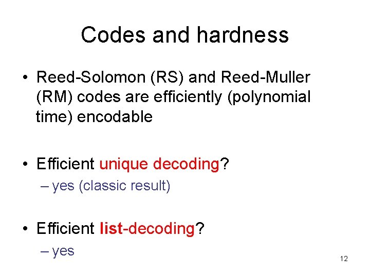
Codes and hardness • Reed-Solomon (RS) and Reed-Muller (RM) codes are efficiently (polynomial time) encodable • Efficient unique decoding? – yes (classic result) • Efficient list-decoding? – yes 12

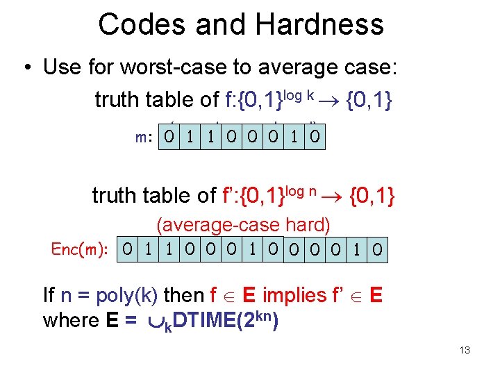
Codes and Hardness • Use for worst-case to average case: truth table of f: {0, 1}log k {0, 1} m: 0(worst-case 1 1 0 0 0 hard) 1 0 truth table of f’: {0, 1}log n {0, 1} (average-case hard) Enc(m): 0 1 1 0 0 0 0 1 0 If n = poly(k) then f E implies f’ E where E = k. DTIME(2 kn) 13

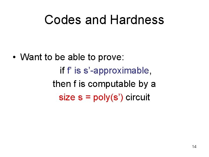
Codes and Hardness • Want to be able to prove: if f’ is s’-approximable, then f is computable by a size s = poly(s’) circuit 14

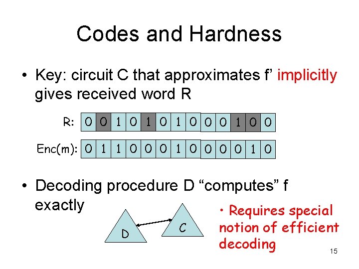
Codes and Hardness • Key: circuit C that approximates f’ implicitly gives received word R R: 0 0 1 0 1 0 0 Enc(m): 0 1 1 0 0 0 0 1 0 • Decoding procedure D “computes” f exactly • Requires special D C notion of efficient decoding 15

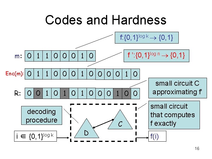
Codes and Hardness f: {0, 1}log k {0, 1} f ’: {0, 1}log n {0, 1} m: 0 1 1 0 0 0 1 0 Enc(m): 0 1 1 0 0 0 0 1 0 R: 0 0 1 0 1 0 0 decoding procedure i ∈ {0, 1}log k D C small circuit C approximating f’ small circuit that computes f exactly f(i) 16

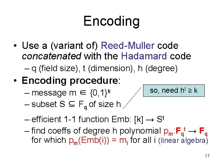
Encoding • Use a (variant of) Reed-Muller code concatenated with the Hadamard code – q (field size), t (dimension), h (degree) • Encoding procedure: – message m ∈ – subset S ⊆ Fq of size h {0, 1}k so, need ht ≥ k – efficient 1 -1 function Emb: [k] → St – find coeffs of degree h polynomial pm: Fqt → Fq for which pm(Emb(i)) = mi for all i (linear algebra) 17

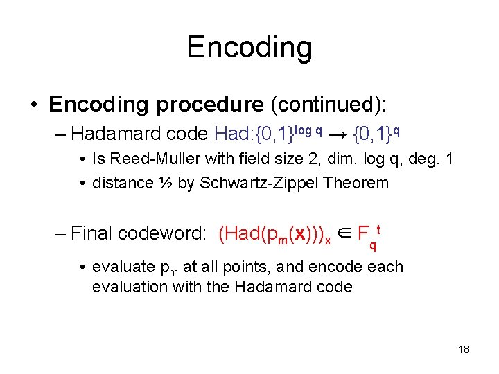
Encoding • Encoding procedure (continued): – Hadamard code Had: {0, 1}log q → {0, 1}q • Is Reed-Muller with field size 2, dim. log q, deg. 1 • distance ½ by Schwartz-Zippel Theorem – Final codeword: (Had(pm(x)))x ∈ Fqt • evaluate pm at all points, and encode each evaluation with the Hadamard code 18

Encoding m: 0 1 1 0 0 0 1 0 F qt Emb: [k] → St St 5 2 7 1 2 9 0 3 6 8 3 pm degree h polynomial with pm(Emb(i)) = mi evaluate at all x ∈ Fqt encode each symbol. . . 0 1 0 1 0. . . with Had: {0, 1}log q→ {0, 1}q 19

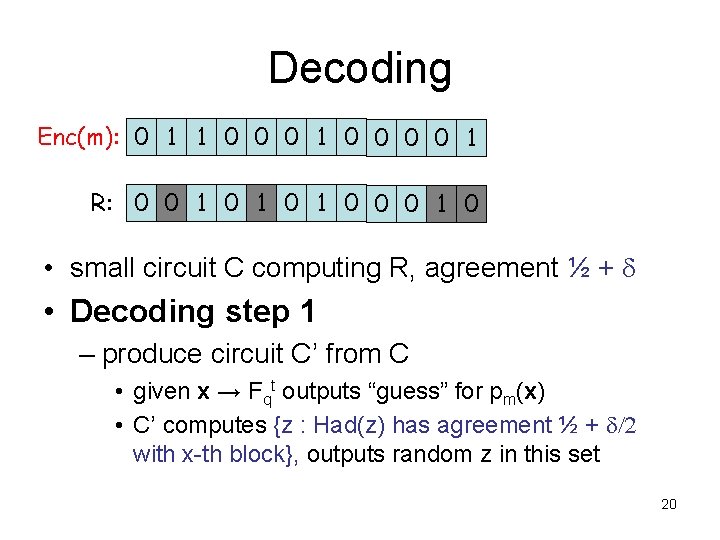
Decoding Enc(m): 0 1 1 0 0 0 0 1 R: 0 0 1 0 1 0 0 0 1 0 • small circuit C computing R, agreement ½ + • Decoding step 1 – produce circuit C’ from C • given x → Fqt outputs “guess” for pm(x) • C’ computes {z : Had(z) has agreement ½ + /2 with x-th block}, outputs random z in this set 20

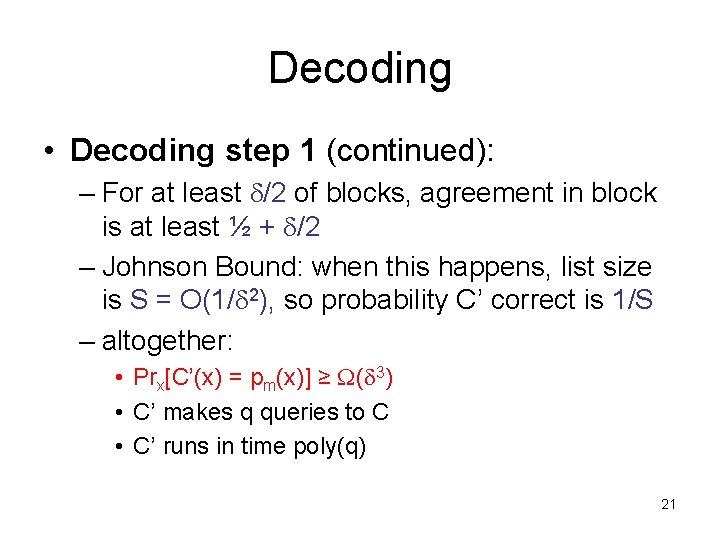
Decoding • Decoding step 1 (continued): – For at least /2 of blocks, agreement in block is at least ½ + /2 – Johnson Bound: when this happens, list size is S = O(1/ 2), so probability C’ correct is 1/S – altogether: • Prx[C’(x) = pm(x)] ≥ ( 3) • C’ makes q queries to C • C’ runs in time poly(q) 21

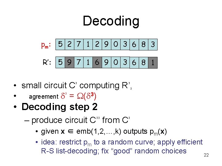
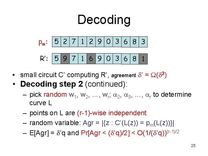
Decoding pm: 5 2 7 1 2 9 0 3 6 8 3 R’: 5 9 7 1 6 9 0 3 6 8 1 • small circuit C’ computing R’, • agreement ’ = ( 3) • Decoding step 2 – produce circuit C’’ from C’ • given x ∈ emb(1, 2, …, k) outputs pm(x) • idea: restrict pm to a random curve; apply efficient R-S list-decoding; fix “good” random choices 22

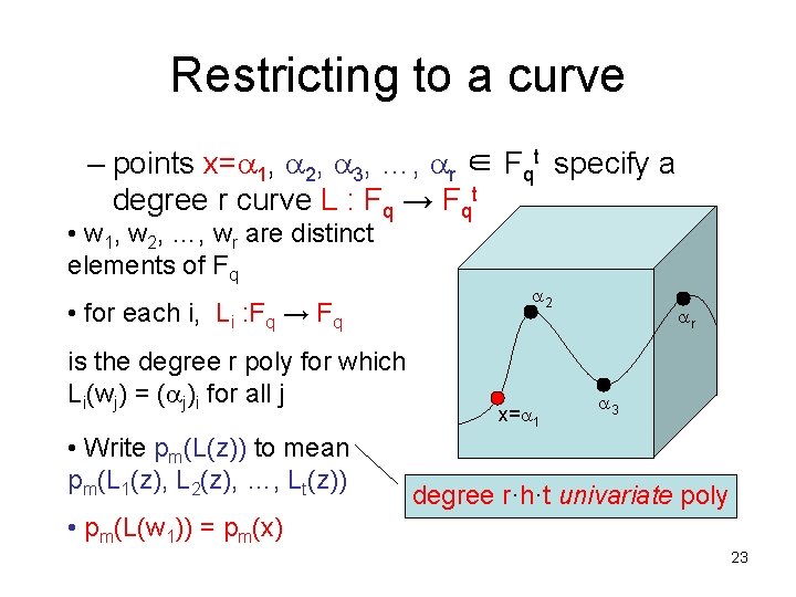
Restricting to a curve – points x= 1, 2, 3, …, r ∈ Fqt specify a degree r curve L : Fq → Fqt • w 1, w 2, …, wr are distinct elements of Fq • for each i, Li : Fq → Fq is the degree r poly for which Li(wj) = ( j)i for all j • Write pm(L(z)) to mean pm(L 1(z), L 2(z), …, Lt(z)) 2 x= 1 r 3 degree r·h·t univariate poly • pm(L(w 1)) = pm(x) 23

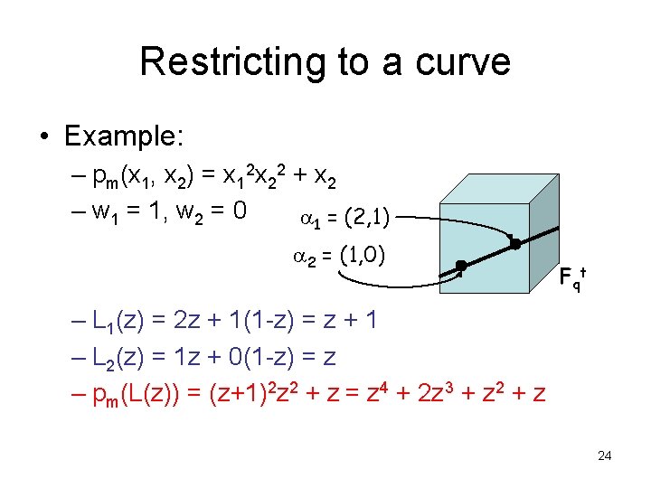
Restricting to a curve • Example: – pm(x 1, x 2) = x 12 x 22 + x 2 – w 1 = 1, w 2 = 0 1 = (2, 1) 2 = (1, 0) F qt – L 1(z) = 2 z + 1(1 -z) = z + 1 – L 2(z) = 1 z + 0(1 -z) = z – pm(L(z)) = (z+1)2 z 2 + z = z 4 + 2 z 3 + z 24

Decoding pm: 5 2 7 1 2 9 0 3 6 8 3 R’: 5 9 7 1 6 9 0 3 6 8 1 • small circuit C’ computing R’, agreement ’ = ( 3) • Decoding step 2 (continued): – pick random w 1, w 2, …, wr; 2, 3, …, r to determine curve L – points on L are (r-1)-wise independent – random variable: Agr = |{z : C’(L(z)) = pm(L(z))}| – E[Agr] = ’q and Pr[Agr < ( ’q)/2] < O(1/( ’q))(r-1)/2 25

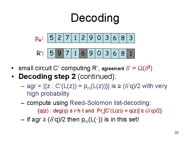
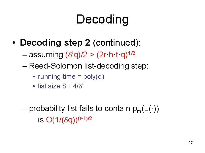
Decoding pm: 5 2 7 1 2 9 0 3 6 8 3 R’: 5 9 7 1 6 9 0 3 6 8 1 • small circuit C’ computing R’, agreement ’ = ( 3) • Decoding step 2 (continued): – agr = |{z : C’(L(z)) = pm(L(z))}| is ≥ ( ’q)/2 with very high probability – compute using Reed-Solomon list-decoding: {q(z) : deg(q) ≤ r·h·t and Prz[C’(L(z)) = q(z)] ≥ ( ’q)/2} – if agr ≥ ( ’q)/2 then pm(L(·)) is in this set! 26

Decoding • Decoding step 2 (continued): – assuming ( ’q)/2 > (2 r·h·t·q)1/2 – Reed-Solomon list-decoding step: • running time = poly(q) • list size S · 4/ ’ – probability list fails to contain pm(L(·)) is O(1/( q))(r-1)/2 27

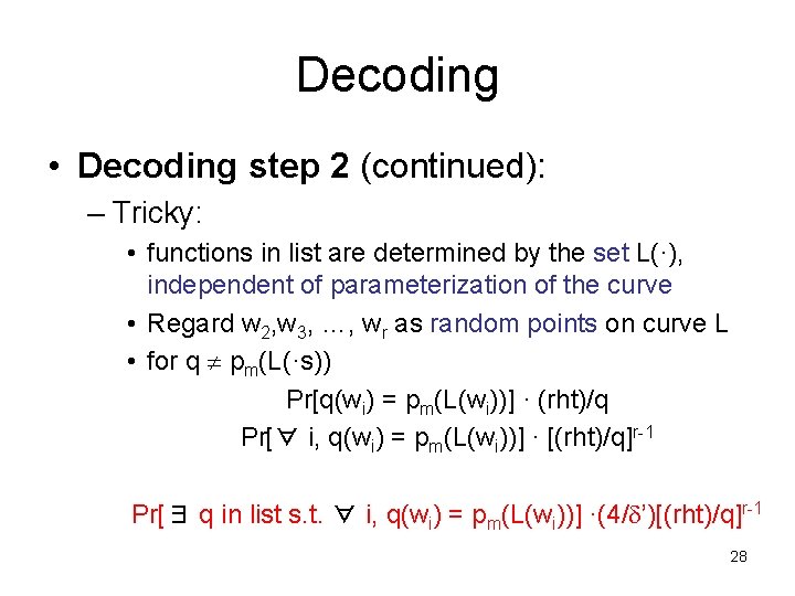
Decoding • Decoding step 2 (continued): – Tricky: • functions in list are determined by the set L(·), independent of parameterization of the curve • Regard w 2, w 3, …, wr as random points on curve L • for q pm(L(·s)) Pr[q(wi) = pm(L(wi))] · (rht)/q Pr[∀ i, q(wi) = pm(L(wi))] · [(rht)/q]r-1 Pr[∃ q in list s. t. ∀ i, q(wi) = pm(L(wi))] ·(4/ ’)[(rht)/q]r-1 28

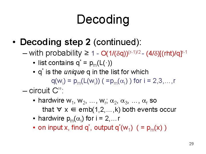
Decoding • Decoding step 2 (continued): – with probability ≥ 1 - O(1/( q))(r-1)/2 - (4/ )[(rht)/q]r-1 • list contains q* = pm(L(·)) • q* is the unique q in the list for which q(wi) = pm(L(wi)) ( =pm( i) ) for i = 2, 3, …, r – circuit C’’: • hardwire w 1, w 2, …, wr; 2, 3, …, r so that ∀ x ∈ emb(1, 2, …, k) both events occur • hardwire pm( i) for i = 2, …r • on input x, find q*, output q*(w 1) ( = pm(x) ) 29

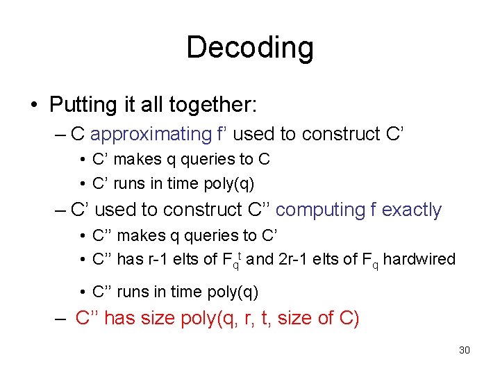
Decoding • Putting it all together: – C approximating f’ used to construct C’ • C’ makes q queries to C • C’ runs in time poly(q) – C’ used to construct C’’ computing f exactly • C’’ makes q queries to C’ • C’’ has r-1 elts of Fqt and 2 r-1 elts of Fq hardwired • C’’ runs in time poly(q) – C’’ has size poly(q, r, t, size of C) 30

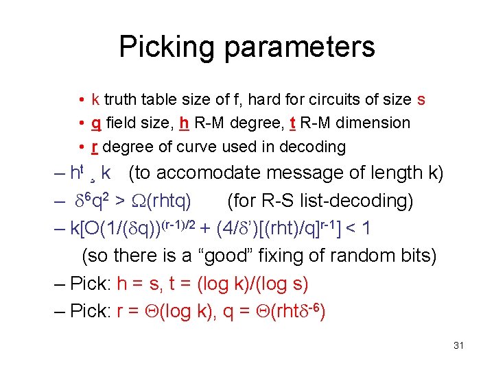
Picking parameters • k truth table size of f, hard for circuits of size s • q field size, h R-M degree, t R-M dimension • r degree of curve used in decoding – ht ¸ k (to accomodate message of length k) – 6 q 2 > (rhtq) (for R-S list-decoding) – k[O(1/( q))(r-1)/2 + (4/ ’)[(rht)/q]r-1] < 1 (so there is a “good” fixing of random bits) – Pick: h = s, t = (log k)/(log s) – Pick: r = (log k), q = (rht -6) 31

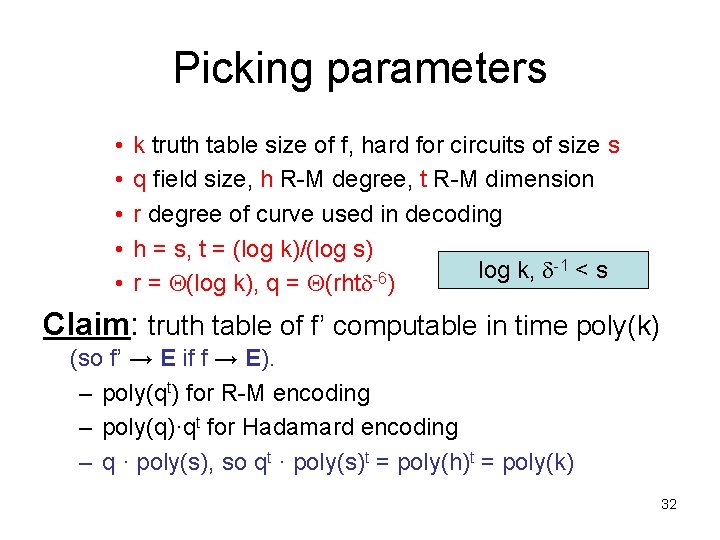
Picking parameters • • • k truth table size of f, hard for circuits of size s q field size, h R-M degree, t R-M dimension r degree of curve used in decoding h = s, t = (log k)/(log s) log k, -1 < s -6 r = (log k), q = (rht ) Claim: truth table of f’ computable in time poly(k) (so f’ → E if f → E). – poly(qt) for R-M encoding – poly(q)·qt for Hadamard encoding – q · poly(s), so qt · poly(s)t = poly(h)t = poly(k) 32

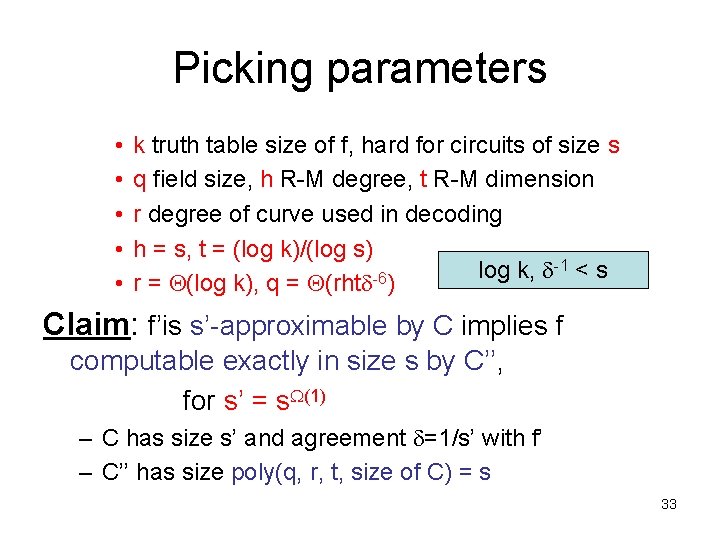
Picking parameters • • • k truth table size of f, hard for circuits of size s q field size, h R-M degree, t R-M dimension r degree of curve used in decoding h = s, t = (log k)/(log s) log k, -1 < s -6 r = (log k), q = (rht ) Claim: f’is s’-approximable by C implies f computable exactly in size s by C’’, for s’ = s (1) – C has size s’ and agreement =1/s’ with f’ – C’’ has size poly(q, r, t, size of C) = s 33

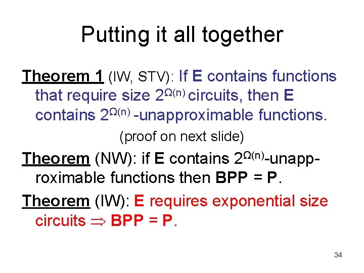
Putting it all together Theorem 1 (IW, STV): If E contains functions that require size 2Ω(n) circuits, then E contains 2Ω(n) -unapproximable functions. (proof on next slide) Theorem (NW): if E contains 2Ω(n)-unapproximable functions then BPP = P. Theorem (IW): E requires exponential size circuits BPP = P. 34

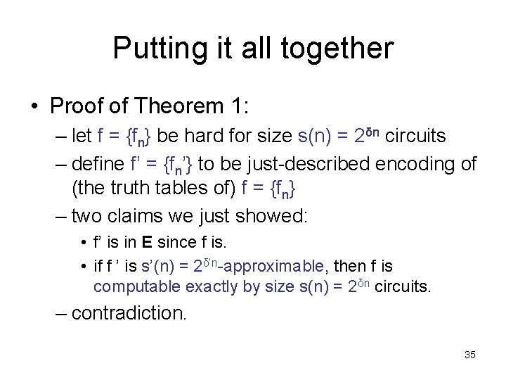
Putting it all together • Proof of Theorem 1: – let f = {fn} be hard for size s(n) = 2δn circuits – define f’ = {fn’} to be just-described encoding of (the truth tables of) f = {fn} – two claims we just showed: • f’ is in E since f is. • if f ’ is s’(n) = 2δ’n-approximable, then f is computable exactly by size s(n) = 2δn circuits. – contradiction. 35