Umans Complexity Theory Lectures Introduction to Randomized Complexity

Umans Complexity Theory Lectures Introduction to Randomized Complexity: - Randomized complexity classes, - Error reduction, -BPP in P/poly -Reingold’s Undirected Graph Reachability in RL

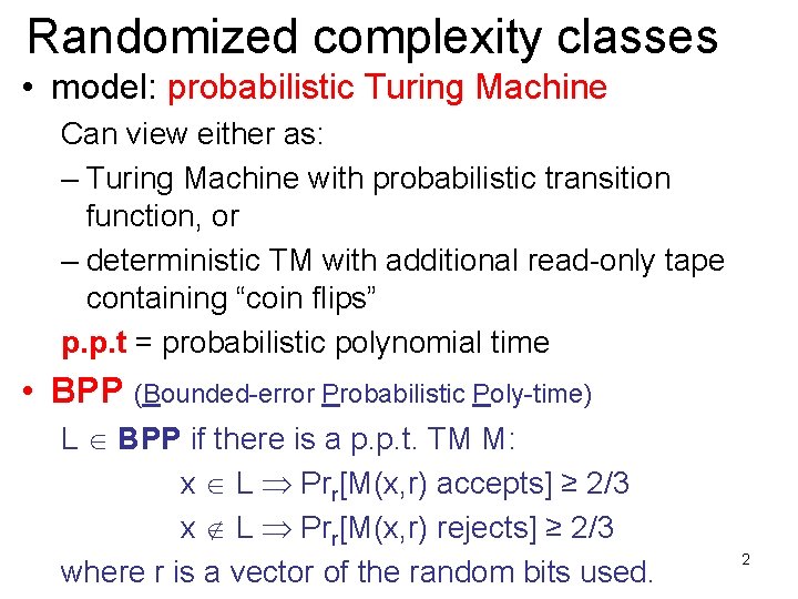
Randomized complexity classes • model: probabilistic Turing Machine Can view either as: – Turing Machine with probabilistic transition function, or – deterministic TM with additional read-only tape containing “coin flips” p. p. t = probabilistic polynomial time • BPP (Bounded-error Probabilistic Poly-time) L BPP if there is a p. p. t. TM M: x L Prr[M(x, r) accepts] ≥ 2/3 x L Prr[M(x, r) rejects] ≥ 2/3 where r is a vector of the random bits used. 2

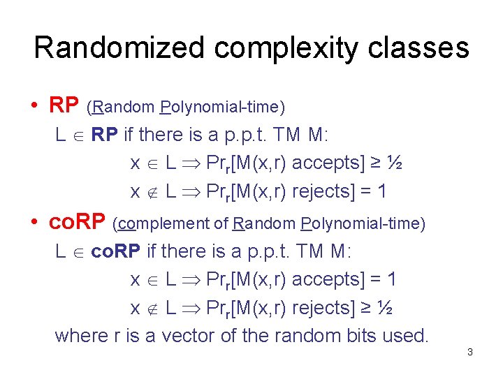
Randomized complexity classes • RP (Random Polynomial-time) L RP if there is a p. p. t. TM M: x L Prr[M(x, r) accepts] ≥ ½ x L Prr[M(x, r) rejects] = 1 • co. RP (complement of Random Polynomial-time) L co. RP if there is a p. p. t. TM M: x L Prr[M(x, r) accepts] = 1 x L Prr[M(x, r) rejects] ≥ ½ where r is a vector of the random bits used. 3

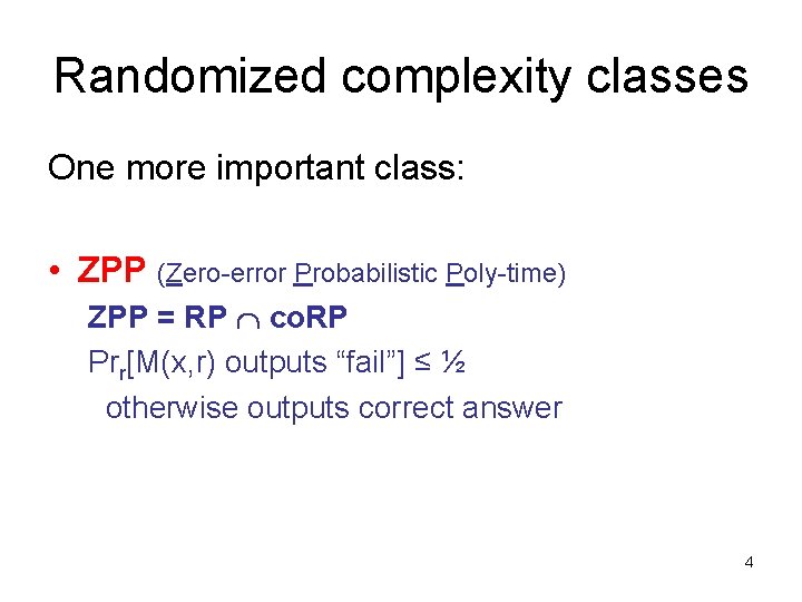
Randomized complexity classes One more important class: • ZPP (Zero-error Probabilistic Poly-time) ZPP = RP co. RP Prr[M(x, r) outputs “fail”] ≤ ½ otherwise outputs correct answer 4

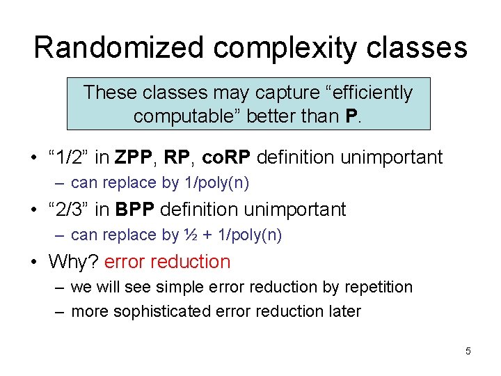
Randomized complexity classes These classes may capture “efficiently computable” better than P. • “ 1/2” in ZPP, RP, co. RP definition unimportant – can replace by 1/poly(n) • “ 2/3” in BPP definition unimportant – can replace by ½ + 1/poly(n) • Why? error reduction – we will see simple error reduction by repetition – more sophisticated error reduction later 5

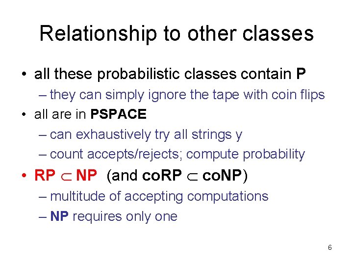
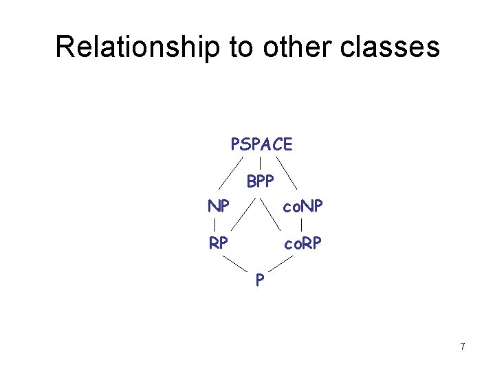
Relationship to other classes • all these probabilistic classes contain P – they can simply ignore the tape with coin flips • all are in PSPACE – can exhaustively try all strings y – count accepts/rejects; compute probability • RP NP (and co. RP co. NP) – multitude of accepting computations – NP requires only one 6

Relationship to other classes PSPACE BPP NP co. NP RP co. RP P 7

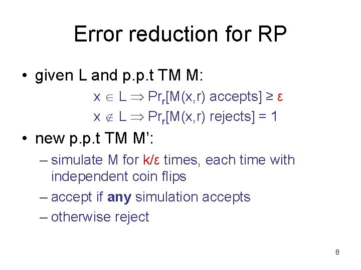
Error reduction for RP • given L and p. p. t TM M: x L Prr[M(x, r) accepts] ≥ ε x L Prr[M(x, r) rejects] = 1 • new p. p. t TM M’: – simulate M for k/ε times, each time with independent coin flips – accept if any simulation accepts – otherwise reject 8

Error reduction for RP x L Prr[M(x, r) accepts] ≥ ε x L Prr[M(x, r) rejects] = 1 • if x L: – probability a given simulation “bad” ≤ (1 – ε) – Since (1–ε)(1/ε) ≤ e-1 we have: – probability all simulations “bad” ≤ (1–ε)(k/ε) ≤ e-k Prr’[M’(x, r’) accepts] ≥ 1 – e-k • if x L: Prr’[M’(x, r’) rejects] = 1 9

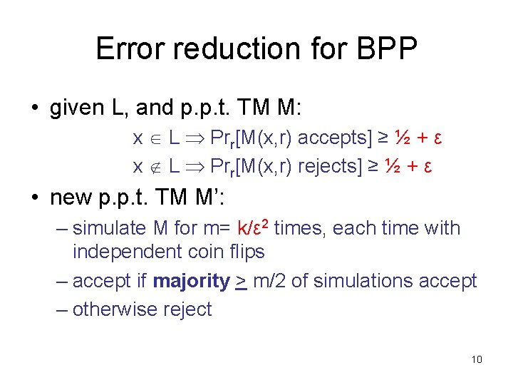
Error reduction for BPP • given L, and p. p. t. TM M: x L Prr[M(x, r) accepts] ≥ ½ + ε x L Prr[M(x, r) rejects] ≥ ½ + ε • new p. p. t. TM M’: – simulate M for m= k/ε 2 times, each time with independent coin flips – accept if majority > m/2 of simulations accept – otherwise reject 10

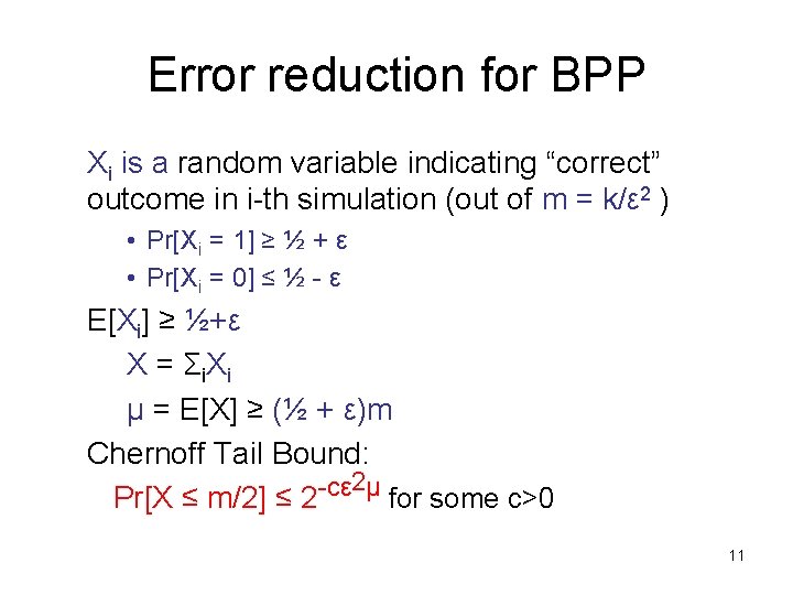
Error reduction for BPP Xi is a random variable indicating “correct” outcome in i-th simulation (out of m = k/ε 2 ) • Pr[Xi = 1] ≥ ½ + ε • Pr[Xi = 0] ≤ ½ - ε E[Xi] ≥ ½+ε X = Σ i. X i μ = E[X] ≥ (½ + ε)m Chernoff Tail Bound: 2μ -cε Pr[X ≤ m/2] ≤ 2 for some c>0 11

Error reduction for BPP x L Prr[M(x, r) accepts] ≥ ½ + ε x L Prr[M(x, r) rejects] ≥ ½ + ε if x L Prr’[M’(x, r’) accepts] ≥ 1 – (½)ck if x L Prr’[M’(x, r’) rejects] ≥ 1 – (½)ck 12

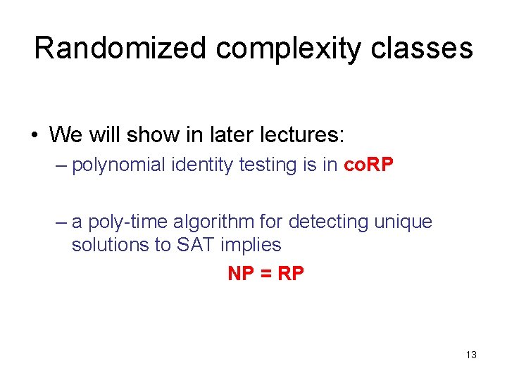
Randomized complexity classes • We will show in later lectures: – polynomial identity testing is in co. RP – a poly-time algorithm for detecting unique solutions to SAT implies NP = RP 13

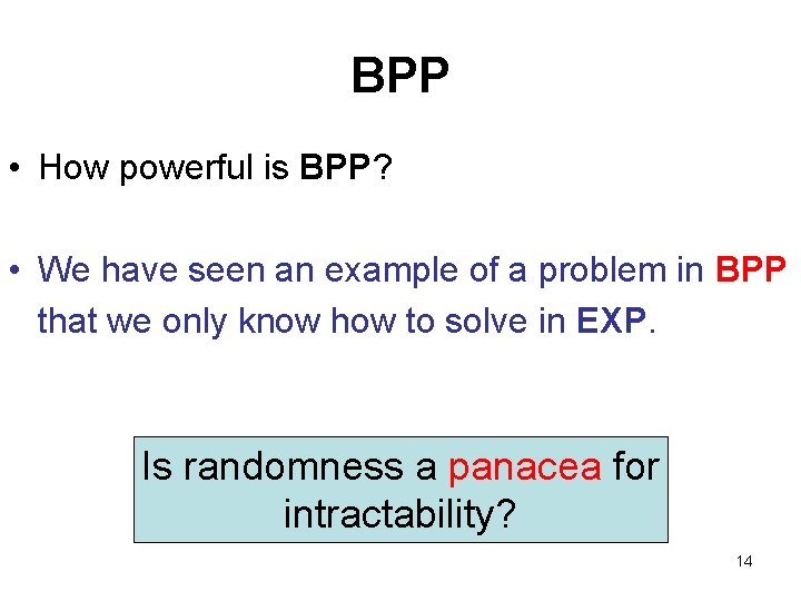
BPP • How powerful is BPP? • We have seen an example of a problem in BPP that we only know how to solve in EXP. Is randomness a panacea for intractability? 14

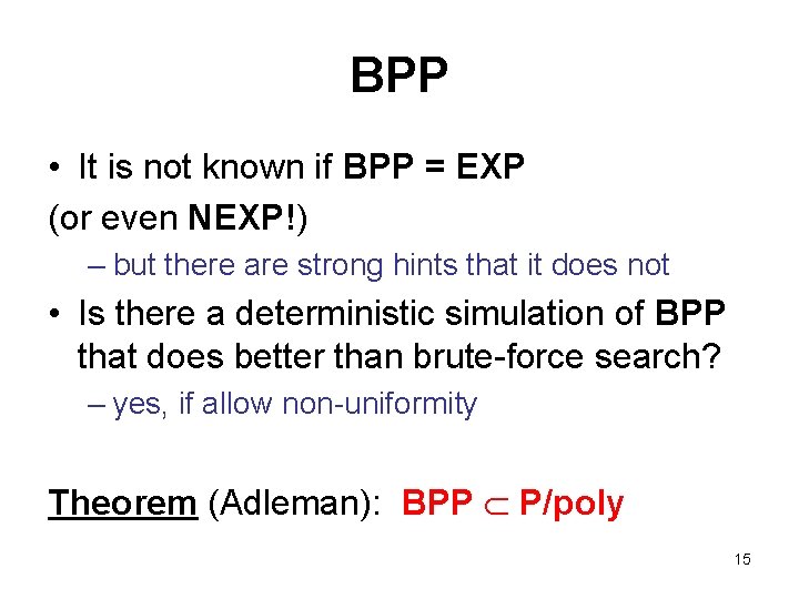
BPP • It is not known if BPP = EXP (or even NEXP!) – but there are strong hints that it does not • Is there a deterministic simulation of BPP that does better than brute-force search? – yes, if allow non-uniformity Theorem (Adleman): BPP P/poly 15

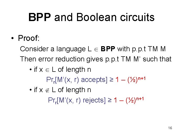
BPP and Boolean circuits • Proof: Consider a language L BPP with p. p. t TM M Then error reduction gives p. p. t TM M’ such that • if x L of length n Prr[M’(x, r) accepts] ≥ 1 – (½)n+1 • if x L of length n Prr[M’(x, r) rejects] ≥ 1 – (½)n+1 16

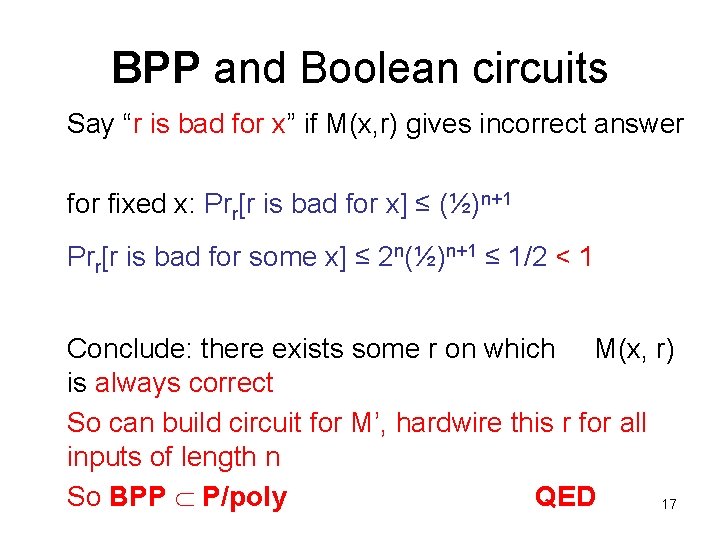
BPP and Boolean circuits Say “r is bad for x” if M(x, r) gives incorrect answer for fixed x: Prr[r is bad for x] ≤ (½)n+1 Prr[r is bad for some x] ≤ 2 n(½)n+1 ≤ 1/2 < 1 Conclude: there exists some r on which M(x, r) is always correct So can build circuit for M’, hardwire this r for all inputs of length n So BPP P/poly QED 17

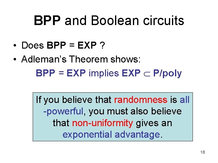
BPP and Boolean circuits • Does BPP = EXP ? • Adleman’s Theorem shows: BPP = EXP implies EXP P/poly If you believe that randomness is all -powerful, you must also believe that non-uniformity gives an exponential advantage. 18

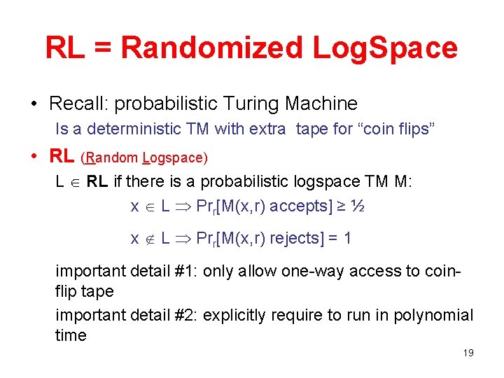
RL = Randomized Log. Space • Recall: probabilistic Turing Machine Is a deterministic TM with extra tape for “coin flips” • RL (Random Logspace) L RL if there is a probabilistic logspace TM M: x L Prr[M(x, r) accepts] ≥ ½ x L Prr[M(x, r) rejects] = 1 important detail #1: only allow one-way access to coinflip tape important detail #2: explicitly require to run in polynomial time 19

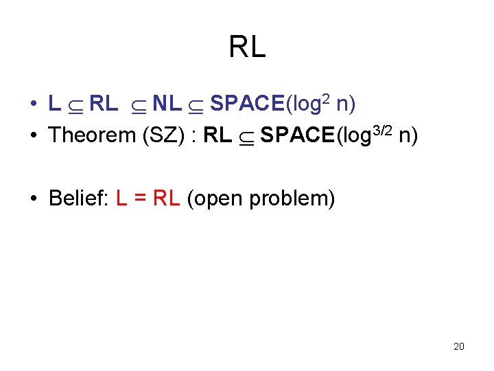
RL • L RL NL SPACE(log 2 n) • Theorem (SZ) : RL SPACE(log 3/2 n) • Belief: L = RL (open problem) 20

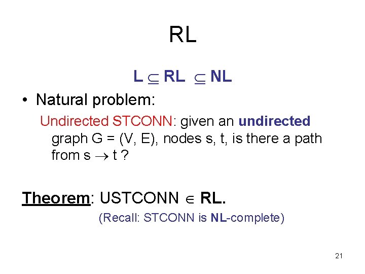
RL L RL NL • Natural problem: Undirected STCONN: given an undirected graph G = (V, E), nodes s, t, is there a path from s t ? Theorem: USTCONN RL. (Recall: STCONN is NL-complete) 21

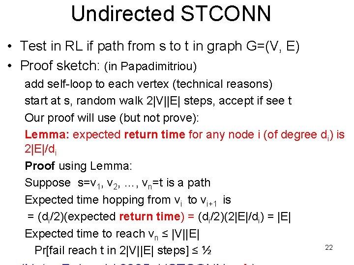
Undirected STCONN • Test in RL if path from s to t in graph G=(V, E) • Proof sketch: (in Papadimitriou) add self-loop to each vertex (technical reasons) start at s, random walk 2|V||E| steps, accept if see t Our proof will use (but not prove): Lemma: expected return time for any node i (of degree di) is 2|E|/di Proof using Lemma: Suppose s=v 1, v 2, …, vn=t is a path Expected time hopping from vi to vi+1 is = (di/2)(expected return time) = (di/2)(2|E|/di) = |E| Expected time to reach vn ≤ |V||E| 22 Pr[fail reach t in 2|V||E| steps] ≤ ½