Transformations Data Cleaning Linear nonlinear transformations 2 kinds

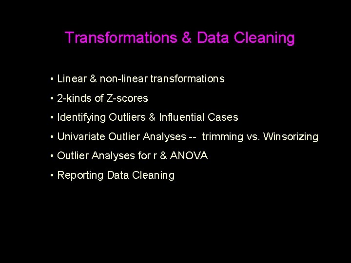
Transformations & Data Cleaning • Linear & non-linear transformations • 2 -kinds of Z-scores • Identifying Outliers & Influential Cases • Univariate Outlier Analyses -- trimming vs. Winsorizing • Outlier Analyses for r & ANOVA • Reporting Data Cleaning

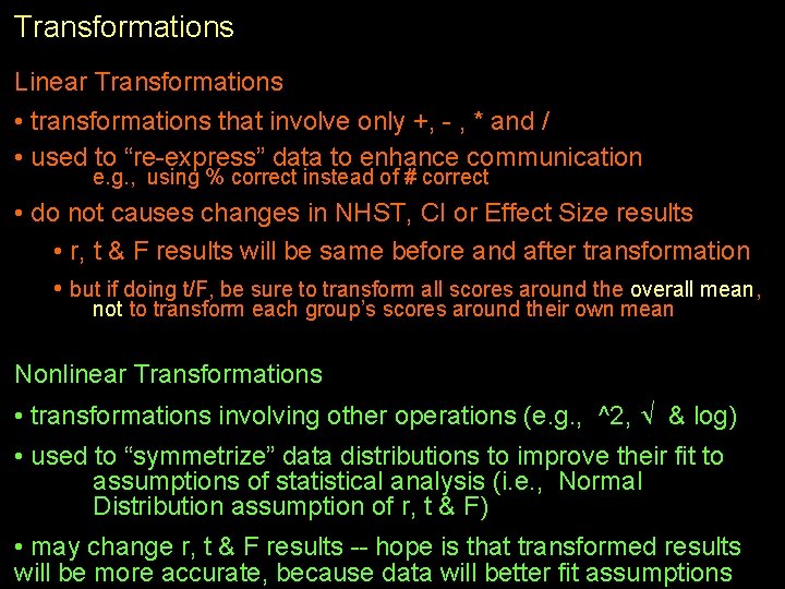
Transformations Linear Transformations • transformations that involve only +, - , * and / • used to “re-express” data to enhance communication e. g. , using % correct instead of # correct • do not causes changes in NHST, CI or Effect Size results • r, t & F results will be same before and after transformation • but if doing t/F, be sure to transform all scores around the overall mean, not to transform each group’s scores around their own mean Nonlinear Transformations • transformations involving other operations (e. g. , ^2, & log) • used to “symmetrize” data distributions to improve their fit to assumptions of statistical analysis (i. e. , Normal Distribution assumption of r, t & F) • may change r, t & F results -- hope is that transformed results will be more accurate, because data will better fit assumptions

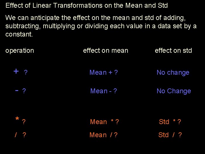
Effect of Linear Transformations on the Mean and Std We can anticipate the effect on the mean and std of adding, subtracting, multiplying or dividing each value in a data set by a constant. operation effect on mean effect on std + ? Mean + ? No change - ? Mean - ? No Change *? Mean * ? Std * ? / ? Mean / ? Std / ?

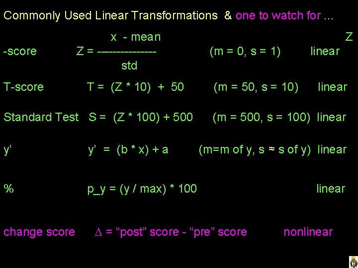
Commonly Used Linear Transformations & one to watch for. . . -score T-score x - mean Z = -------std T = (Z * 10) + 50 Standard Test S = (Z * 100) + 500 y’ y’ = (b * x) + a % p_y = (y / max) * 100 change score Z (m = 0, s = 1) linear (m = 50, s = 10) linear (m = 500, s = 100) linear (m=m of y, s ≈ s of y) linear = “post” score - “pre” score linear nonlinear

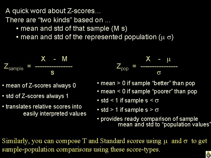
A quick word about Z-scores… There are “two kinds” based on. . . • mean and std of that sample (M s) • mean and std of the represented population ( ) Zsample X - M = --------s • mean of Z-scores always 0 • std of Z-scores always 1 • translates relative scores into easily interpreted values Zpop X - = -------- • mean > 0 if sample “better” than pop • mean < 0 if sample “poorer” than pop • std < 1 if sample s < • std > 1 if sample s > • provides ready comparison of sample mean and std to “population values” Similarly, you can compose T and Standard scores using and to get sample-population comparisons using these score-types.

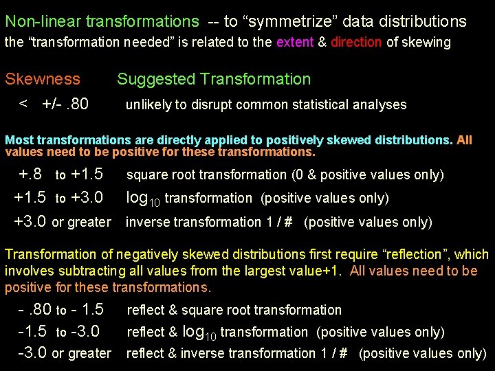
Non-linear transformations -- to “symmetrize” data distributions the “transformation needed” is related to the extent & direction of skewing Skewness < +/-. 80 Suggested Transformation unlikely to disrupt common statistical analyses Most transformations are directly applied to positively skewed distributions. All values need to be positive for these transformations. +. 8 to +1. 5 square root transformation (0 & positive values only) +1. 5 to +3. 0 log 10 transformation (positive values only) +3. 0 or greater inverse transformation 1 / # (positive values only) Transformation of negatively skewed distributions first require “reflection”, which involves subtracting all values from the largest value+1. All values need to be positive for these transformations. -. 80 to - 1. 5 reflect & square root transformation -1. 5 to -3. 0 reflect & log 10 transformation (positive values only) -3. 0 or greater reflect & inverse transformation 1 / # (positive values only)

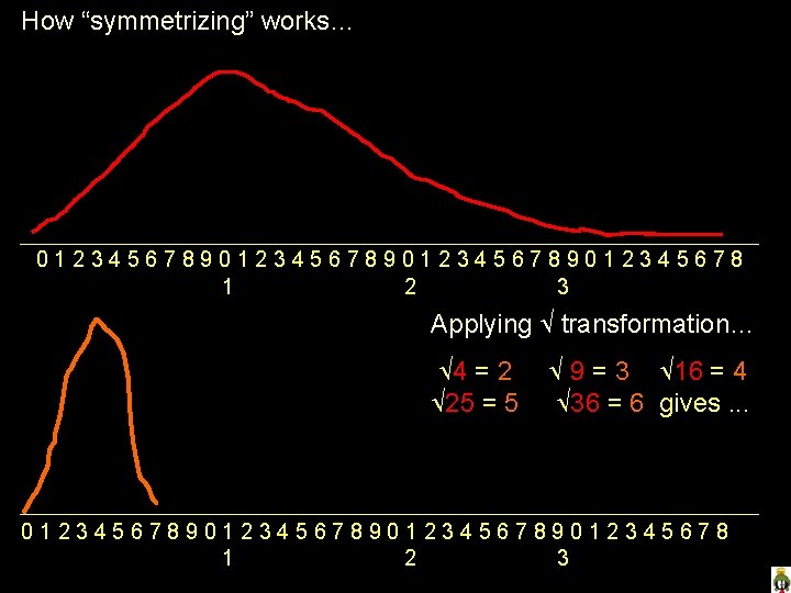
How “symmetrizing” works… 01234567890123456789012345678 1 2 3 Applying transformation… 4 = 2 25 = 5 9 = 3 16 = 4 36 = 6 gives. . . 01234567890123456789012345678 1 2 3

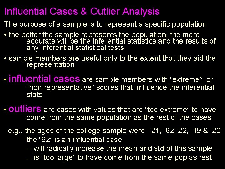
Influential Cases & Outlier Analysis The purpose of a sample is to represent a specific population • the better the sample represents the population, the more accurate will be the inferential statistics and the results of any inferential statistical tests • sample members are useful only to the extent that they aid the representation • influential cases are sample members with “extreme” or “non-representative” scores that influence the inferential stats • outliers are cases with values that are “too extreme” to have come from the same population as the rest of the cases e. g. , the ages of the college sample were 21, 62, 22, 19 & 20 the “ 62” is an influential case -- will radically increase the mean and std of this sample -- is “too large” to have come from the same pop as rest

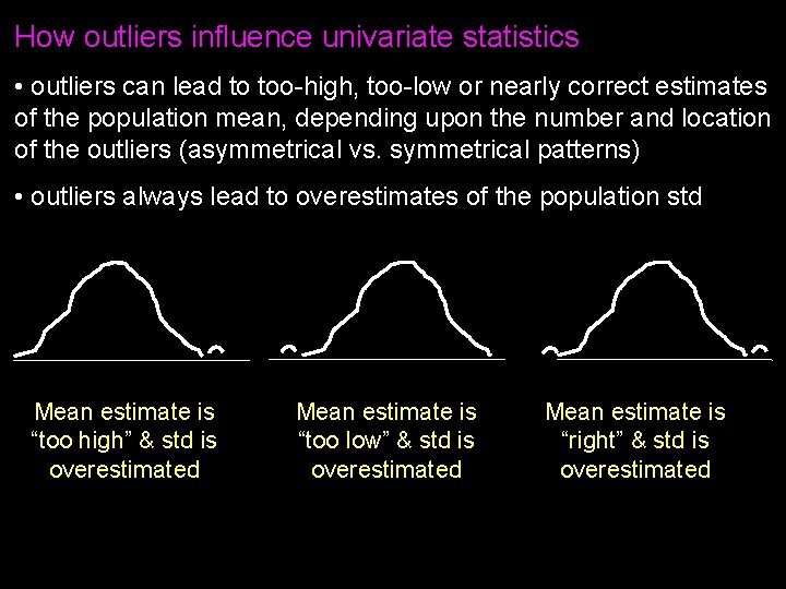
How outliers influence univariate statistics • outliers can lead to too-high, too-low or nearly correct estimates of the population mean, depending upon the number and location of the outliers (asymmetrical vs. symmetrical patterns) • outliers always lead to overestimates of the population std Mean estimate is “too high” & std is overestimated Mean estimate is “too low” & std is overestimated Mean estimate is “right” & std is overestimated

Identifying Outliers for removal The preferred technique is to be able to identify participants who are not likely to be members of the population of interest. However, often the only indication we have that a participant doesn’t come from the population of interest is that they have an “outlying score”. So, we will operate under the assumption that “outlying scores” mean that: 1) a participant is probably not a member of the target population (or that something “bad” happened to their score) 2) if included the data as is would produce a biased estimate of the population value (e. g. , mean, std, r, F, etc. ) and so, should not be included in the data analysis. Key -- application of the approach must be “hypothesis blind”

Statistical Identification of Outliers One common procedure was to identify as outliers any data point with a Z-value greater than 2. 0 (2. 5 & 3. 0 were also common suggestions) • this means that some values that really do belong to the distribution were incorrectly identified as outliers, but simulation and real-data research suggested that statistical estimates were better and more replicable when these procedures were used. • one problem with this approach is that outliers influence the std (making it larger than it should be) leading us to miss outliers (yep – outliers can “hide themselves” when this approach is used) The most common approach used currently is to base outlier analyses on rank-order statistics, which are much less influenced by the outliers they are trying to identify.

Outlier Identification formulas The formula is very simple (easier using SPSS)… Lower bound value = Lower hinge – 1. 5 (hinge spread) Upper bound value = Upper hinge + 1. 5 (hinge spread) Any data value smaller than the lower bound or larger than the upper bound is deemed an outlier – a value that probably doesn’t come from the same population as the other values in the sample. Hoaglin, D. C. , Mosteller, F. , & Tukey, J. W. (1983). Understanding Robust and Exploratory Data Analysis. New York: Wiley. What we do with identified outliers • Trimming – eliminating the data value from the analyses • leads to loss of data, statistical power, etc. ) • Winsorizing – recode the data value to the “nearest acceptable” value (upper or lower bound value) • large/small values are still present, but won’t unduly influence statistical estimates & maintains sample size

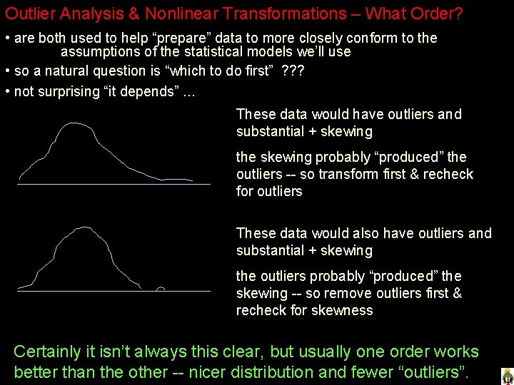
Outlier Analysis & Nonlinear Transformations – What Order? • are both used to help “prepare” data to more closely conform to the assumptions of the statistical models we’ll use • so a natural question is “which to do first” ? ? ? • not surprising “it depends”. . . These data would have outliers and substantial + skewing the skewing probably “produced” the outliers -- so transform first & recheck for outliers These data would also have outliers and substantial + skewing the outliers probably “produced” the skewing -- so remove outliers first & recheck for skewness Certainly it isn’t always this clear, but usually one order works better than the other -- nicer distribution and fewer “outliers”.

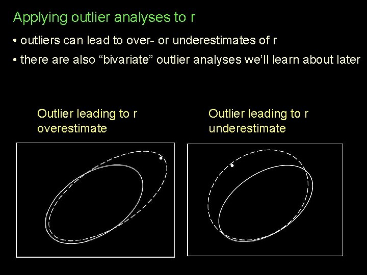
Applying outlier analyses to r • outliers can lead to over- or underestimates of r • there also “bivariate” outlier analyses we’ll learn about later Outlier leading to r overestimate Outlier leading to r underestimate

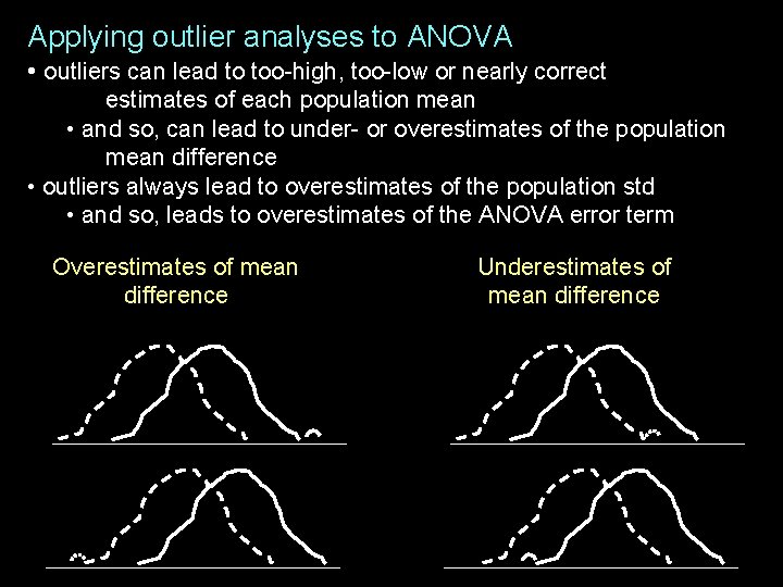
Applying outlier analyses to ANOVA • outliers can lead to too-high, too-low or nearly correct estimates of each population mean • and so, can lead to under- or overestimates of the population mean difference • outliers always lead to overestimates of the population std • and so, leads to overestimates of the ANOVA error term Overestimates of mean difference Underestimates of mean difference

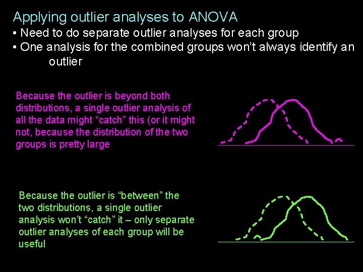
Applying outlier analyses to ANOVA • Need to do separate outlier analyses for each group • One analysis for the combined groups won’t always identify an outlier Because the outlier is beyond both distributions, a single outlier analysis of all the data might “catch” this (or it might not, because the distribution of the two groups is pretty large Because the outlier is “between” the two distributions, a single outlier analysis won’t “catch” it – only separate outlier analyses of each group will be useful

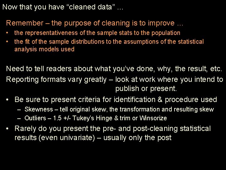
Now that you have “cleaned data” … Remember – the purpose of cleaning is to improve … • the representativeness of the sample stats to the population • the fit of the sample distributions to the assumptions of the statistical analysis models used Need to tell readers about what you’ve done, why, the result, etc. Reporting formats vary greatly – look at work where you intend to publish or present. • Be sure to present criteria for identification & procedure used – Skewness – tell original skew, the transformation and resulting skew – Outliers – 1. 5 +/- Tukey’s Hinge & trim or Winsorize • Rarely do you present the pre- and post-cleaning statistical results (even univariate) – usually only the post