Topic 8 Money Interest Rates and Exchange Rates

Topic 8 Money, Interest Rates, and Exchange Rates Slides prepared by Thomas Bishop Copyright © 2009 Pearson Addison-Wesley. All rights reserved.

Preview • What is money? • Control of the supply of money • The willingness to hold money • A model of money and interest rates • A model of money, interest rates, and exchange rates • Long run effects of changes in money supply on prices, interest rates, and exchange rates Copyright © 2009 Pearson Addison-Wesley. All rights reserved. 2

Introduction • In the next three lectures, we will build a macroeconomic model that links exchange rates, interest rates, inflation rates, and output. • Begin by examining how the supply and demand for money affects interest rates and exchange rates. Copyright © 2009 Pearson Addison-Wesley. All rights reserved. 3

What Is Money? • It is a medium of exchange: a generally accepted means of payment. ¨ Money eliminates the enormous search costs connected with a barter system. • Money is a unit of account: a widely recognized measure of value. • It is an asset or a store of value. ¨ Money is the most liquid of all assets because it can be transformed into goods and services rapidly without high transactions costs. Copyright © 2009 Pearson Addison-Wesley. All rights reserved. 4

What Is Money? (cont. ) • Money is currency and bank deposits on which checks can be written. • Money supply in this class will be M 1: the total amount of currency and checking deposits held by households and firms. ¨ In 2006, the U. S. total money supply was $1. 39 trillion (or 10. 5% of GNP). Copyright © 2009 Pearson Addison-Wesley. All rights reserved. 5

Money Supply • An economy’s money supply is controlled by its central bank. • In the US, the central banking system is the Federal Reserve System. ¨ It directly regulates the amount of currency in circulation. And it indirectly controls the amount of checking deposits issued by private banks. • For now, we assume that the central bank simply sets the size of the money supply at the level it desires. Copyright © 2009 Pearson Addison-Wesley. All rights reserved. 6

Money Demand • Money demand represents the amount of money (currency and checking deposits) that people are willing to hold (instead of less liquid assets like government bonds, a large time deposit, or real estate). ¨ What influences willingness to hold money? ¨ We consider individual demand for money and aggregate demand for money. Copyright © 2009 Pearson Addison-Wesley. All rights reserved. 7

What Influences Demand for Money by Individuals and Institutions? • Individuals base their demand for any asset (including money) on three characteristics: 1. Expected return (or interest rates): the difference in rates of return between money and less liquid assets is reflected by the market interest rate. • A rise in the interest rate raises the cost of holding money (rather than interest-paying assets) and causes money demand to fall. Copyright © 2009 Pearson Addison-Wesley. All rights reserved. 8

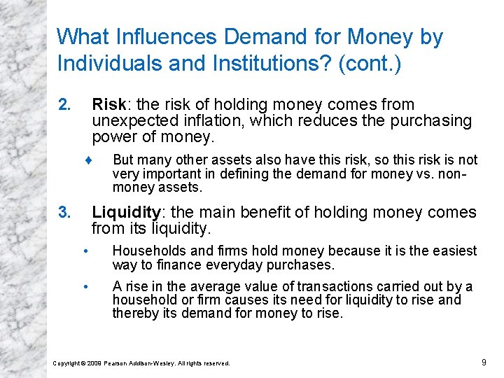
What Influences Demand for Money by Individuals and Institutions? (cont. ) 2. Risk: the risk of holding money comes from unexpected inflation, which reduces the purchasing power of money. ¨ 3. But many other assets also have this risk, so this risk is not very important in defining the demand for money vs. nonmoney assets. Liquidity: the main benefit of holding money comes from its liquidity. • Households and firms hold money because it is the easiest way to finance everyday purchases. • A rise in the average value of transactions carried out by a household or firm causes its need for liquidity to rise and thereby its demand for money to rise. Copyright © 2009 Pearson Addison-Wesley. All rights reserved. 9

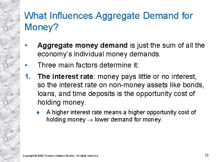
What Influences Aggregate Demand for Money? • Aggregate money demand is just the sum of all the economy’s individual money demands. • Three main factors determine it: 1. The interest rate: money pays little or no interest, so the interest rate on non-money assets like bonds, loans, and time deposits is the opportunity cost of holding money. ¨ A higher interest rate means a higher opportunity cost of holding money lower demand for money. Copyright © 2009 Pearson Addison-Wesley. All rights reserved. 10

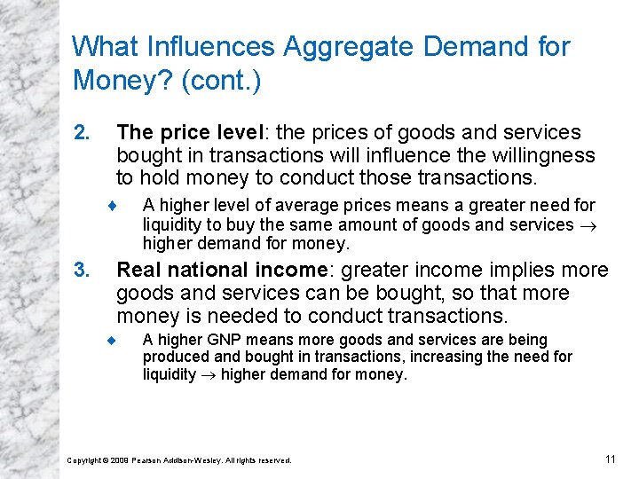
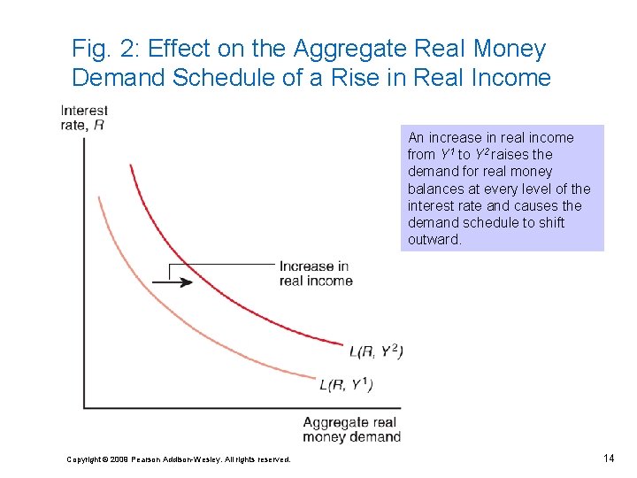
What Influences Aggregate Demand for Money? (cont. ) 2. The price level: the prices of goods and services bought in transactions will influence the willingness to hold money to conduct those transactions. ¨ 3. A higher level of average prices means a greater need for liquidity to buy the same amount of goods and services higher demand for money. Real national income: greater income implies more goods and services can be bought, so that more money is needed to conduct transactions. ¨ A higher GNP means more goods and services are being produced and bought in transactions, increasing the need for liquidity higher demand for money. Copyright © 2009 Pearson Addison-Wesley. All rights reserved. 11

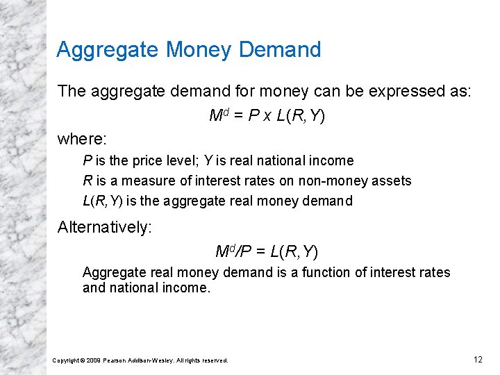
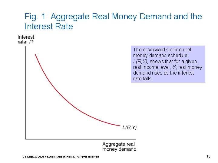
Aggregate Money Demand The aggregate demand for money can be expressed as: Md = P x L(R, Y) where: P is the price level; Y is real national income R is a measure of interest rates on non-money assets L(R, Y) is the aggregate real money demand Alternatively: Md/P = L(R, Y) Aggregate real money demand is a function of interest rates and national income. Copyright © 2009 Pearson Addison-Wesley. All rights reserved. 12

Fig. 1: Aggregate Real Money Demand the Interest Rate The downward sloping real money demand schedule, L(R, Y), shows that for a given real income level, Y, real money demand rises as the interest rate falls. Copyright © 2009 Pearson Addison-Wesley. All rights reserved. 13

Fig. 2: Effect on the Aggregate Real Money Demand Schedule of a Rise in Real Income An increase in real income from Y 1 to Y 2 raises the demand for real money balances at every level of the interest rate and causes the demand schedule to shift outward. Copyright © 2009 Pearson Addison-Wesley. All rights reserved. 14

A Model of the Money Market • The money market is in equilibrium when the money supply set by the central bank equals aggregate money demand. • We examine how the interest rate is determined by money market equilibrium, given the price level and output, both of which are temporarily assumed to be unaffected by monetary changes. Copyright © 2009 Pearson Addison-Wesley. All rights reserved. 15

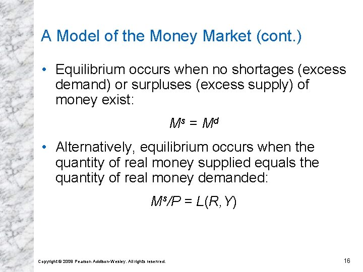
A Model of the Money Market (cont. ) • Equilibrium occurs when no shortages (excess demand) or surpluses (excess supply) of money exist: Ms = Md • Alternatively, equilibrium occurs when the quantity of real money supplied equals the quantity of real money demanded: Ms/P = L(R, Y) Copyright © 2009 Pearson Addison-Wesley. All rights reserved. 16

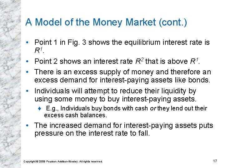
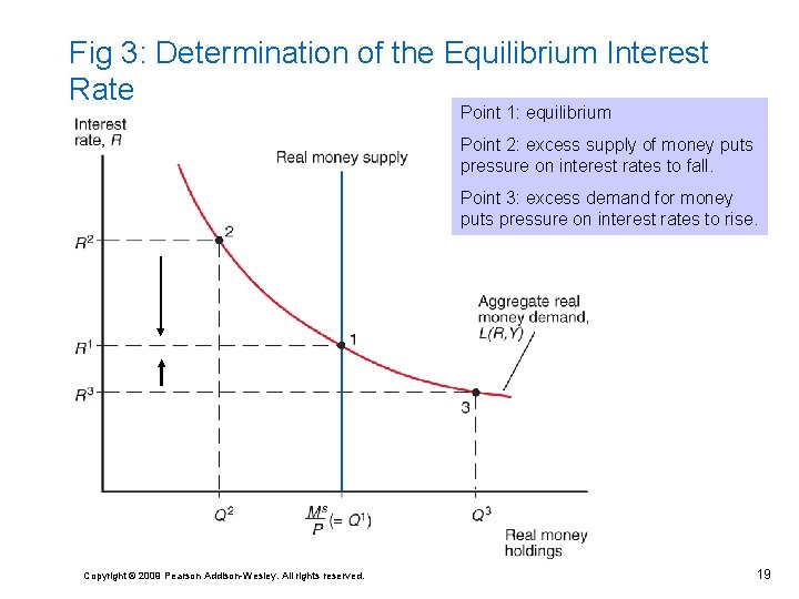
A Model of the Money Market (cont. ) • Point 1 in Fig. 3 shows the equilibrium interest rate is R 1. • Point 2 shows an interest rate R 2 that is above R 1. • There is an excess supply of money and therefore an excess demand for interest-paying assets like bonds. • Individuals will attempt to reduce their liquidity by using some money to buy interest-paying assets. ¨ E. g. , Individuals buy bonds with cash or they lend out their excess cash balances. • The increased demand for interest-paying assets puts pressure on the interest rate to fall. Copyright © 2009 Pearson Addison-Wesley. All rights reserved. 17

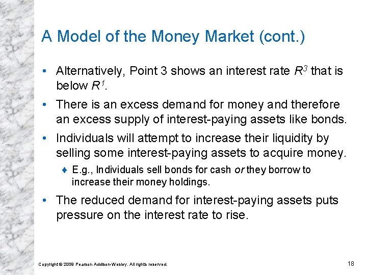
A Model of the Money Market (cont. ) • Alternatively, Point 3 shows an interest rate R 3 that is below R 1. • There is an excess demand for money and therefore an excess supply of interest-paying assets like bonds. • Individuals will attempt to increase their liquidity by selling some interest-paying assets to acquire money. ¨ E. g. , Individuals sell bonds for cash or they borrow to increase their money holdings. • The reduced demand for interest-paying assets puts pressure on the interest rate to rise. Copyright © 2009 Pearson Addison-Wesley. All rights reserved. 18

Fig 3: Determination of the Equilibrium Interest Rate Point 1: equilibrium Point 2: excess supply of money puts pressure on interest rates to fall. Point 3: excess demand for money puts pressure on interest rates to rise. Copyright © 2009 Pearson Addison-Wesley. All rights reserved. 19

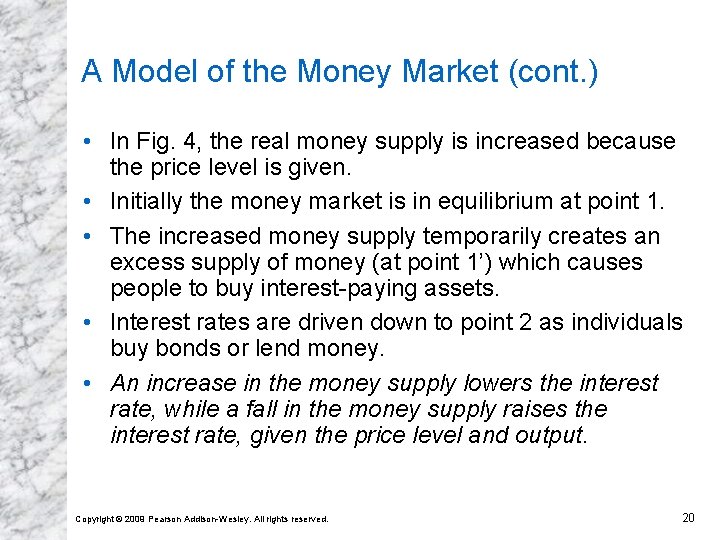
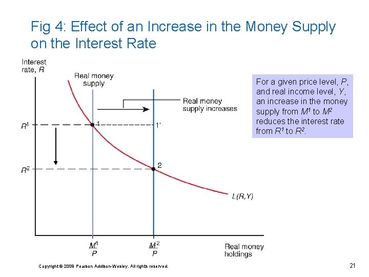
A Model of the Money Market (cont. ) • In Fig. 4, the real money supply is increased because the price level is given. • Initially the money market is in equilibrium at point 1. • The increased money supply temporarily creates an excess supply of money (at point 1’) which causes people to buy interest-paying assets. • Interest rates are driven down to point 2 as individuals buy bonds or lend money. • An increase in the money supply lowers the interest rate, while a fall in the money supply raises the interest rate, given the price level and output. Copyright © 2009 Pearson Addison-Wesley. All rights reserved. 20

Fig 4: Effect of an Increase in the Money Supply on the Interest Rate 1’ Copyright © 2009 Pearson Addison-Wesley. All rights reserved. For a given price level, P, and real income level, Y, an increase in the money supply from M 1 to M 2 reduces the interest rate from R 1 to R 2. 21

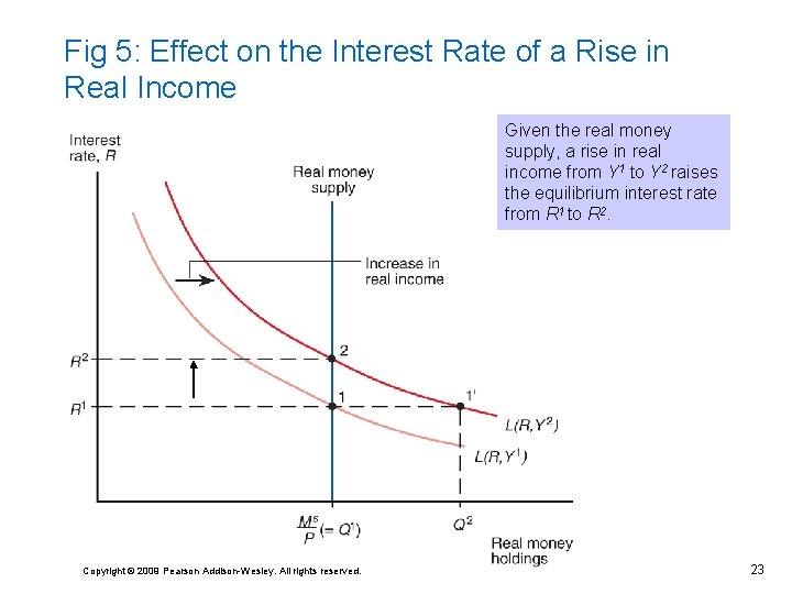
A Model of the Money Market (cont. ) • In Fig. 5, an increase in output (holding MS and P fixed) leads to an increase in aggregate real money demand. • Initially the money market is in equilibrium at point 1. • The increased money demand temporarily creates an excess demand for money (at point 1’) which causes interest rates to rise (to point 2). • An increase in real output raises the interest rate, while a fall in real output lowers the interest rate, given the price level and the money supply. Copyright © 2009 Pearson Addison-Wesley. All rights reserved. 22

Fig 5: Effect on the Interest Rate of a Rise in Real Income Given the real money supply, a rise in real income from Y 1 to Y 2 raises the equilibrium interest rate from R 1 to R 2. Copyright © 2009 Pearson Addison-Wesley. All rights reserved. 23

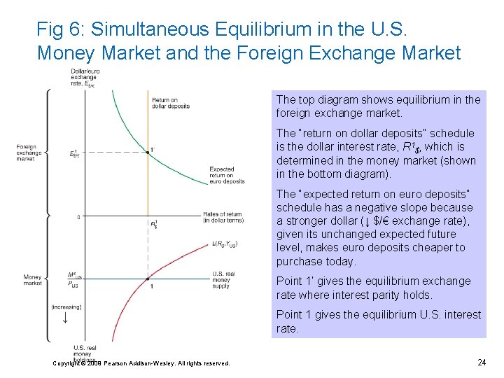
Fig 6: Simultaneous Equilibrium in the U. S. Money Market and the Foreign Exchange Market The top diagram shows equilibrium in the foreign exchange market. The “return on dollar deposits” schedule is the dollar interest rate, R 1$, which is determined in the money market (shown in the bottom diagram). The “expected return on euro deposits” schedule has a negative slope because a stronger dollar (↓ $/€ exchange rate), given its unchanged expected future level, makes euro deposits cheaper to purchase today. Point 1’ gives the equilibrium exchange rate where interest parity holds. Point 1 gives the equilibrium U. S. interest rate. Copyright © 2009 Pearson Addison-Wesley. All rights reserved. 24

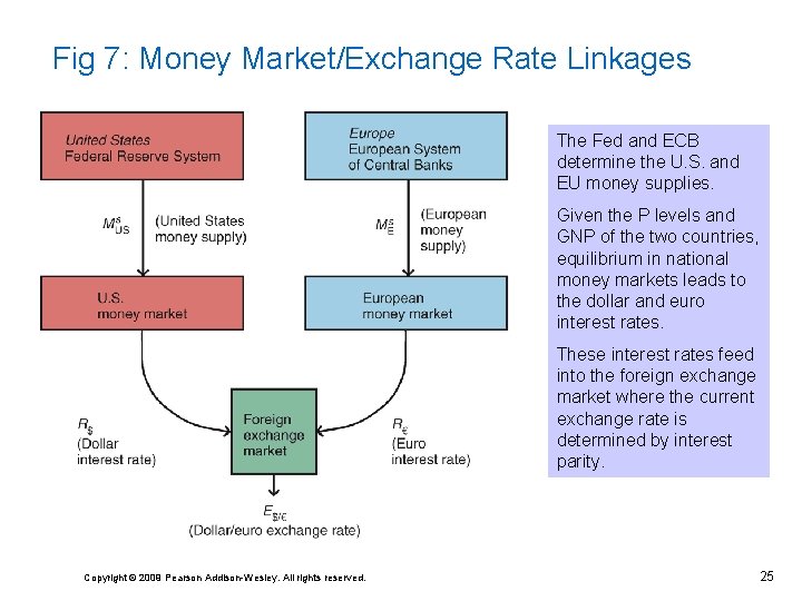
Fig 7: Money Market/Exchange Rate Linkages The Fed and ECB determine the U. S. and EU money supplies. Given the P levels and GNP of the two countries, equilibrium in national money markets leads to the dollar and euro interest rates. These interest rates feed into the foreign exchange market where the current exchange rate is determined by interest parity. Copyright © 2009 Pearson Addison-Wesley. All rights reserved. 25

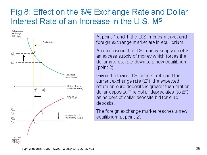
Fig 8: Effect on the $/€ Exchange Rate and Dollar Interest Rate of an Increase in the U. S. MS At point 1 and 1’ the U. S. money market and foreign exchange market are in equilibrium. An increase in the U. S. money supply creates an excess supply of money which forces the dollar interest rate down to a new equilibrium (point 2). Given the lower U. S. interest rate and the current exchange rate (E 1), the expected return on euro deposits is greater than that on dollar deposits. The dollar depreciates (to E 2) as holders of dollar deposits bid for euro deposits. The foreign exchange market reaches a new equilibrium at point 2’. Copyright © 2009 Pearson Addison-Wesley. All rights reserved. 26

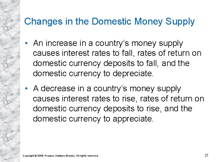
Changes in the Domestic Money Supply • An increase in a country’s money supply causes interest rates to fall, rates of return on domestic currency deposits to fall, and the domestic currency to depreciate. • A decrease in a country’s money supply causes interest rates to rise, rates of return on domestic currency deposits to rise, and the domestic currency to appreciate. Copyright © 2009 Pearson Addison-Wesley. All rights reserved. 27

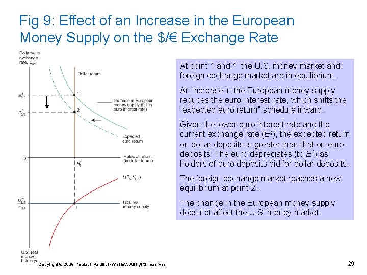
Changes in the Foreign Money Supply • How would an increase in the supply of euros affect the U. S. money market and foreign exchange markets? • An increase in the supply of euros reduces interest rates in the EU, reducing the expected rate of return on euro deposits. • This reduction in the expected rate of return on euro deposits causes the euro to depreciate. • We predict no change in the U. S. money market due to the change in the supply of euros. Copyright © 2009 Pearson Addison-Wesley. All rights reserved. 28

Fig 9: Effect of an Increase in the European Money Supply on the $/€ Exchange Rate At point 1 and 1’ the U. S. money market and foreign exchange market are in equilibrium. An increase in the European money supply reduces the euro interest rate, which shifts the “expected euro return” schedule inward. Given the lower euro interest rate and the current exchange rate (E 1), the expected return on dollar deposits is greater than that on euro deposits. The euro depreciates (to E 2) as holders of euro deposits bid for dollar deposits. The foreign exchange market reaches a new equilibrium at point 2’. The change in the European money supply does not affect the U. S. money market. Copyright © 2009 Pearson Addison-Wesley. All rights reserved. 29

Long Run and Short Run • Our SR analysis of the link between countries’ money markets and foreign exchange markets assumes that price levels and exchange rate expectations were given. • We must now consider how monetary changes work themselves out over the LR –when prices are perfectly flexible and adjust to preserve full employment. Copyright © 2009 Pearson Addison-Wesley. All rights reserved. 30

Long Run and Short Run (cont. ) • In the SR, prices do not have sufficient time to adjust to market conditions. ¨ Our previous analysis has been a SR analysis. • In the LR, prices of factors of production and of output have sufficient time to adjust to market conditions. ¨ Wages adjust to the demand supply of labor. ¨ Real output and income are determined by the amount of workers and other factors of production—by the economy’s productive capacity—not by the quantity of money supplied. ¨ (Real) interest rates depend on the supply of saved funds and the demand for saved funds. Copyright © 2009 Pearson Addison-Wesley. All rights reserved. 31

Long Run and Short Run (cont. ) • In the LR, the quantity of money supplied does not influence the amount of output, (real) interest rates, and therefore the aggregate real money demand, L(R, Y). • However, the quantity of money supplied is predicted to make the level of average prices adjust proportionally in the LR. ¨ The equilibrium condition Ms/P = L(R, Y) shows that P adjusts proportionally when Ms changes because L(R, Y) does not change. Copyright © 2009 Pearson Addison-Wesley. All rights reserved. 32

Long Run and Short Run (cont. ) • E. g. , a doubling of the money supply has the same LR effect as a currency reform in which each unit of “old currency” is replaced by two units of “new currency. ” • If the economy is initially fully employed, every money price eventually doubles, but real GNP, the (real) interest rate, and all relative prices return to their LR levels. Why? • Full-employment GNP is determined by the economy’s endowments of factors, so LR real output does not depend on the money supply. Copyright © 2009 Pearson Addison-Wesley. All rights reserved. 33

Long Run and Short Run (cont. ) • The (real) interest rate is independent of the money supply in the LR. • If the money supply and all prices double permanently, there is no reason why people previously willing to borrow or lend at 10% would not be willing to do so afterward. • Relative prices also remain the same if all money prices double. • Thus, money supply changes do not change the LR allocation of resources! Only the absolute value of money prices change. Copyright © 2009 Pearson Addison-Wesley. All rights reserved. 34

Long Run and Short Run (cont. ) • A doubling of the U. S. money supply would cause the $/€ exchange rate to double. So the U. S. dollar would depreciate by 50% against the euro. • A permanent increase in a country’s money supply causes a proportional LR depreciation of its currency against foreign currencies. Copyright © 2009 Pearson Addison-Wesley. All rights reserved. 35

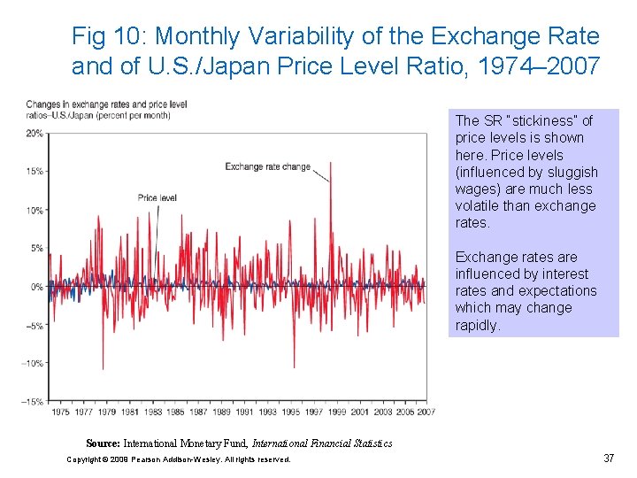
Short-run Price Rigidity • Our SR analysis has assumed that prices (unlike exchange rates) do not change immediately. Why? • Many prices (like wages) are written into long-term contracts and cannot be changed immediately when the money supply changes. • Wages comprise 70% of production costs and therefore strongly influence output prices. • Output prices are “sticky” in the SR because wages are “sticky” in the SR. Copyright © 2009 Pearson Addison-Wesley. All rights reserved. 36

Fig 10: Monthly Variability of the Exchange Rate and of U. S. /Japan Price Level Ratio, 1974– 2007 The SR “stickiness” of price levels is shown here. Price levels (influenced by sluggish wages) are much less volatile than exchange rates. Exchange rates are influenced by interest rates and expectations which may change rapidly. Source: International Monetary Fund, International Financial Statistics Copyright © 2009 Pearson Addison-Wesley. All rights reserved. 37

Money and Prices in the Long Run • Although price levels are sticky in the SR, an increase in the money supply creates immediate demand cost pressures that eventually lead to future increases in the price level. • These pressures come from three main sources. Copyright © 2009 Pearson Addison-Wesley. All rights reserved. 38

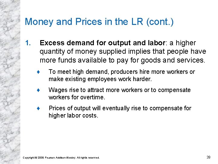
Money and Prices in the LR (cont. ) 1. Excess demand for output and labor: a higher quantity of money supplied implies that people have more funds available to pay for goods and services. ¨ To meet high demand, producers hire more workers or make existing employees work harder. ¨ Wages rise to attract more workers or to compensate workers for overtime. ¨ Prices of output will eventually rise to compensate for higher labor costs. Copyright © 2009 Pearson Addison-Wesley. All rights reserved. 39

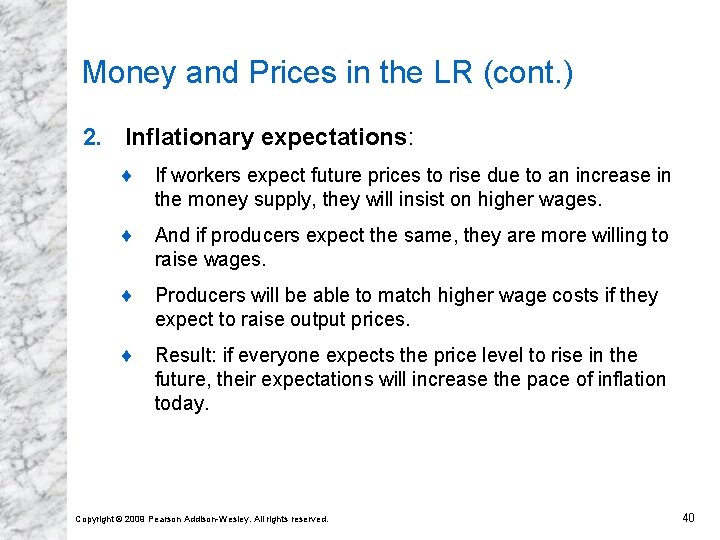
Money and Prices in the LR (cont. ) 2. Inflationary expectations: ¨ If workers expect future prices to rise due to an increase in the money supply, they will insist on higher wages. ¨ And if producers expect the same, they are more willing to raise wages. ¨ Producers will be able to match higher wage costs if they expect to raise output prices. ¨ Result: if everyone expects the price level to rise in the future, their expectations will increase the pace of inflation today. Copyright © 2009 Pearson Addison-Wesley. All rights reserved. 40

Money and Prices in the LR (cont. ) 3. Raw materials prices: • Many raw materials (like oil and metals) used in the production of goods are sold in markets where prices adjust rapidly, even in the SR. • By causing the prices of such materials to jump upward, a money supply increase raises production costs. • Eventually producers will raise output prices to cover their higher materials costs. Copyright © 2009 Pearson Addison-Wesley. All rights reserved. 41

Money, Prices, Exchange Rates, and Expectations • We now apply our analysis of inflation to study the adjustment of the $/€ exchange rate following a permanent increase in the U. S. money supply. • We begin our analysis by assuming that the economy starts with all variables at their long-run levels and that output remains constant as the economy adjusts to the money supply increase. Copyright © 2009 Pearson Addison-Wesley. All rights reserved. 42

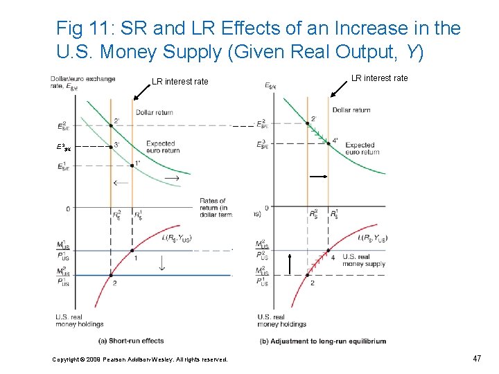
Money, Prices, and Exchange Rates in the Long Run (cont. ) • Fig. 11 shows the SR and LR effects of an increase in the U. S. money supply on the interest rate, price level, and exchange rate. • The LR interest rate is R 1 (point 1). • An increase in the MS at fixed prices (P 1) leads to a higher real MS and thereby a lower SR interest rate, R 2 (at point 2). • The lower interest rate reduces the return on dollar deposits which causes the exchange rate to appreciate (i. e. , the dollar depreciates) from E 1 to E 3 (point 1’ to point 3’). Copyright © 2009 Pearson Addison-Wesley. All rights reserved. 43

Money, Prices, and Exchange Rates in the Long Run (cont. ) • So far we have repeated our earlier SR analysis which held prices and exchange rate expectations fixed. • But people will now expect a LR increase in all dollar prices (including the $/€ exchange rate). • Recall that a rise in the expected future $/€ exchange rate (i. e. , a future euro appreciation) raises the expected dollar return on euro deposits which shifts the “expected euro return” schedule outward. Copyright © 2009 Pearson Addison-Wesley. All rights reserved. 44

Money, Prices, and Exchange Rates in the Long Run (cont. ) • Notice that the dollar depreciation is greater (E 1 to E 2) than it would be if the expected future exchange rate stayed fixed (E 1 to E 3). • If the expected exchange rate did not change, the new SR equilibrium would be at point 3’ rather than point 2’. • Panel (b): the price level begins to rise from P 1 to its new LR level of P 2. • The real money supply has not changed in the LR because the price level has risen in proportion to the increase in the nominal money supply. Copyright © 2009 Pearson Addison-Wesley. All rights reserved. 45

Money, Prices, and Exchange Rates in the Long Run (cont. ) • Since the real money supply has fallen to its initial level, the equilibrium interest rate must increase to R 1 in the LR (point 4). • The dollar appreciates against the euro (from E 2 to E 3) in this adjustment because the U. S. interest rate has increased from R 2 to R 1. • The LR equilibrium exchange rate is E 3 at point 4’. Copyright © 2009 Pearson Addison-Wesley. All rights reserved. 46

Fig 11: SR and LR Effects of an Increase in the U. S. Money Supply (Given Real Output, Y) LR interest rate E 3$/€ Copyright © 2009 Pearson Addison-Wesley. All rights reserved. 47

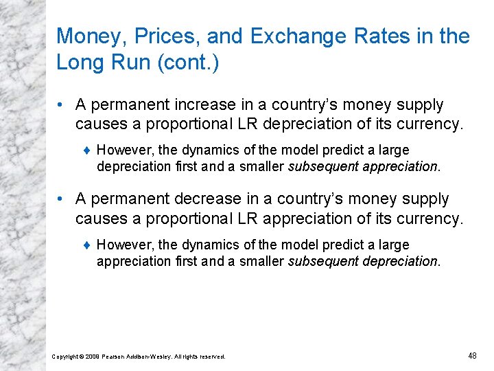
Money, Prices, and Exchange Rates in the Long Run (cont. ) • A permanent increase in a country’s money supply causes a proportional LR depreciation of its currency. ¨ However, the dynamics of the model predict a large depreciation first and a smaller subsequent appreciation. • A permanent decrease in a country’s money supply causes a proportional LR appreciation of its currency. ¨ However, the dynamics of the model predict a large appreciation first and a smaller subsequent depreciation. Copyright © 2009 Pearson Addison-Wesley. All rights reserved. 48

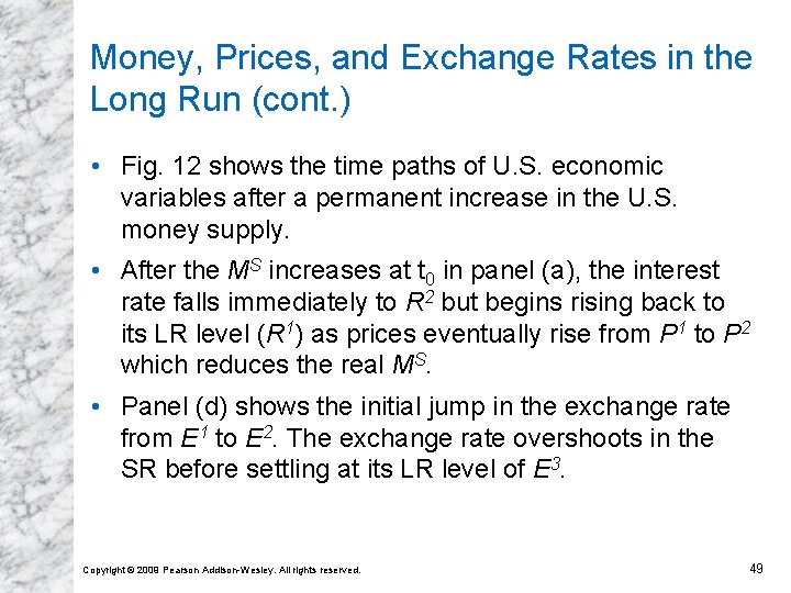
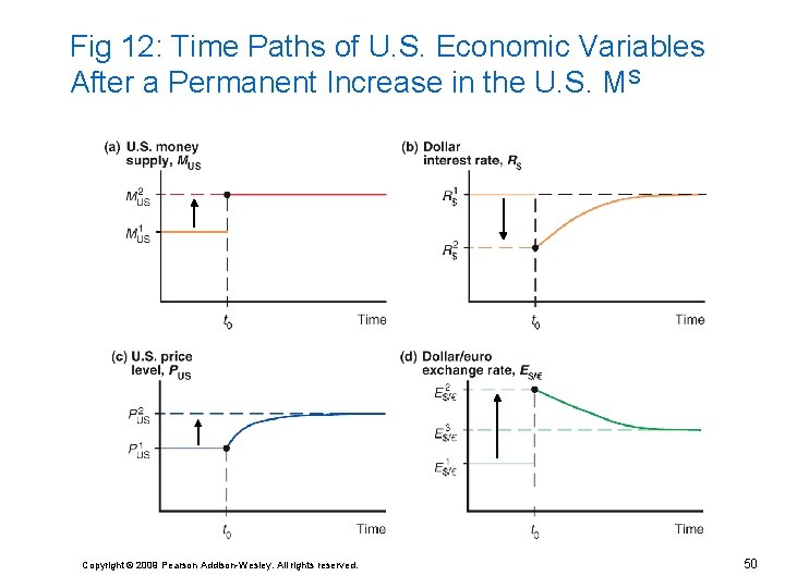
Money, Prices, and Exchange Rates in the Long Run (cont. ) • Fig. 12 shows the time paths of U. S. economic variables after a permanent increase in the U. S. money supply. • After the MS increases at t 0 in panel (a), the interest rate falls immediately to R 2 but begins rising back to its LR level (R 1) as prices eventually rise from P 1 to P 2 which reduces the real MS. • Panel (d) shows the initial jump in the exchange rate from E 1 to E 2. The exchange rate overshoots in the SR before settling at its LR level of E 3. Copyright © 2009 Pearson Addison-Wesley. All rights reserved. 49

Fig 12: Time Paths of U. S. Economic Variables After a Permanent Increase in the U. S. MS Copyright © 2009 Pearson Addison-Wesley. All rights reserved. 50

Exchange Rate Overshooting • The exchange rate is said to overshoot when its immediate response to a change is greater than its LR response. • Overshooting is predicted to occur when monetary policy has an immediate effect on interest rates, but not on prices and (expected) inflation. • Overshooting helps explain why exchange rates are so volatile. • Overshooting is a direct consequence of the SR rigidity of prices. Copyright © 2009 Pearson Addison-Wesley. All rights reserved. 51

Exchange Rate Overshooting (cont. ) • In a pretend world where the price level could adjust immediately to its new LR level after a money supply increase, the dollar interest rate would not fall because prices would adjust immediately to stop the real money supply from rising. • There would be no need for overshooting to maintain equilibrium in the foreign exchange market. • The exchange rate would jump to its new LR equilibrium immediately. Copyright © 2009 Pearson Addison-Wesley. All rights reserved. 52