The Hedonic Pricing Method Part 1 1 Hedonic

The Hedonic Pricing Method Part 1 1

Hedonic pricing method Revealed preferences No questionnaire! We gather data that come from the market No need to build a hypothetical market Where do we decide to live? Why do we choose a specific location? Which factors push companies to choose one location rather than another? Which characteristics of an area affect housing prices? Which are the important elements of a house that determine its price? 2

The choice of localization The choice of housing is a composite good Distance from work, availability of public services, distance from schools, availability of green areas, availability of sport facilities, characteristics of housing (# of bedrooms, # of bathrooms, flat, etc. ) etc. We assume that buyers choose houses that maximize their utility The constraints in the maximization problem are given by income, the price of the houses and the level of taxes => therefore, the housing market give us some information on buyers preferences for housing and for their localization 3

Composite goods In the conjoint analysis and in the multi-site travel cost model we saw that goods (or sites) can be described by a set of attributes or characteristics. The hedonic pricing method uses the same idea that goods are composed by a set of characteristics. Consider the characteristics of a house: Number of floors, presence of a garden, GCH, number of bedrooms, number of bathrooms, square footage of the house, type of house, age, materials, etc. And also: Distance from public transport, distance from the city centre, distance from main roads, distance from shops, distance from sport facilities, crime rate, average income of residents, presence of a university, etc. The composite good has a price, but there is no explicit price for each characteristic that compose the good.

The hedonic pricing method Problem of estimating hedonic equations Hedonic prices are identified through a comparison of similar goods that differ for the quality of one characteristic The basic idea is to use the systematic variation in the price of a good that can be explained by an environmental characteristic of the good. This is the starting point to assess the WTP for the environmental characteristic 5

Example Let’s consider 2 residential properties identical in all characteristics and localization. The only difference is that house A has 2 bedrooms, while house B has 3 bedrooms. In a competitive market, the price difference between the two houses reflects the value of the additional room of house B. If the price difference between the two houses is less than buyers’ WTP for the additional room, then buyers will try to buy house B, driving up its price until the equilibrium is reached. In the same way, if house A costs much less than house B, buyers will increase the demand for house A, driving up its price. 6

The hedonic pricing method applies this simple concept to the environmental characteristics of residential properties The price difference between houses that have different levels of environmental quality, keeping constant all other characteristics, reflects the WTP for the different level of environmental quality => we can assess the value of an environmental quality, according to market prices of residential properties => variation in environmental quality affects the price of housing 7

A bit of history 1926 Waugh studies the variation of prices of vegetables 1938 Court looks at the car market in Detroit 1967 first application to the housing market: Ridker and Henning => effects of air pollution on prices of housing 1974 Rosen describe the first formal model of the hedonic pricing method Other applications: ◦ ◦ Agricultural goods Cars Wine Job market 8

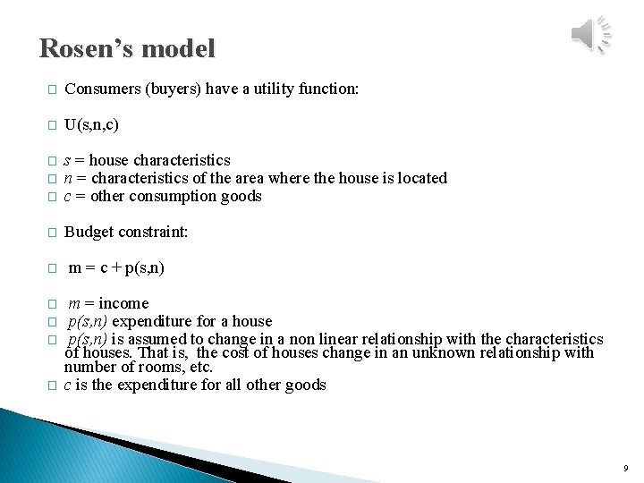
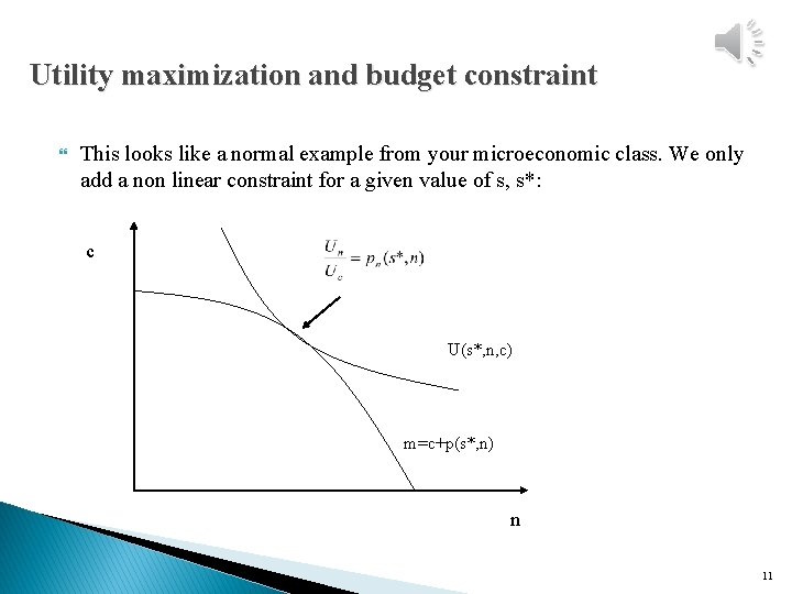
Rosen’s model � Consumers (buyers) have a utility function: � U(s, n, c) � � � s = house characteristics n = characteristics of the area where the house is located c = other consumption goods � Budget constraint: � � � m = c + p(s, n) m = income p(s, n) expenditure for a house p(s, n) is assumed to change in a non linear relationship with the characteristics of houses. That is, the cost of houses change in an unknown relationship with number of rooms, etc. c is the expenditure for all other goods 9

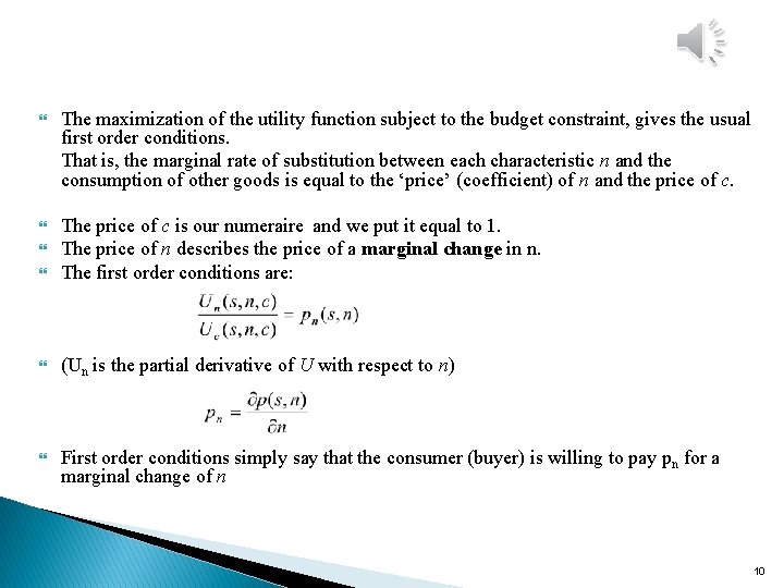
The maximization of the utility function subject to the budget constraint, gives the usual first order conditions. That is, the marginal rate of substitution between each characteristic n and the consumption of other goods is equal to the ‘price’ (coefficient) of n and the price of c. The price of c is our numeraire and we put it equal to 1. The price of n describes the price of a marginal change in n. The first order conditions are: (Un is the partial derivative of U with respect to n) First order conditions simply say that the consumer (buyer) is willing to pay pn for a marginal change of n 10

Utility maximization and budget constraint This looks like a normal example from your microeconomic class. We only add a non linear constraint for a given value of s, s*: c U(s*, n, c) m=c+p(s*, n) n 11

The hedonic price function The function that describes how housing price changes when housing characteristics change: p(s, n) is the hedonic price function The derivative of the function with respect to one of the characteristics n is the ‘implicit price’ of n. If we knew the hedonic price function and the implicit price of n, we could estimate buyers’ WTP for n, given that this is equal to the marginal rate of substitution between n and the other goods (numeracies) 12

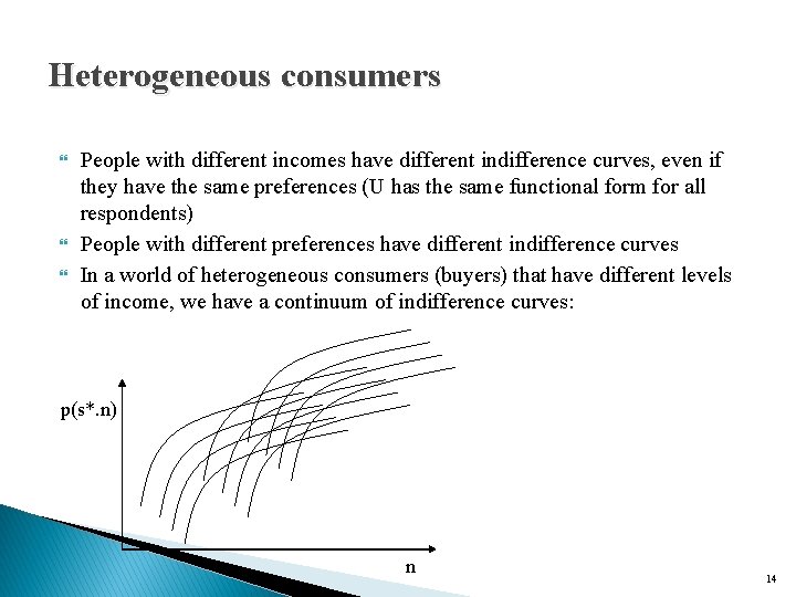
Indifference curves The budget constraint says that we don’t spend for other goods is spent for housing: p(s, n): c = m – p(s, n) The utility function can be written in this way: U(s, n, c)=U(s, n, m – p(s, n)) Therefore we can describe the utility function of consumers (buyers) with indifference curves (for given values of m and s): Each indifference curve gives for a constant level of utility the expenditure on housing and n for a given level of income and s. p(s*. n) U n 13

Heterogeneous consumers People with different incomes have different indifference curves, even if they have the same preferences (U has the same functional form for all respondents) People with different preferences have different indifference curves In a world of heterogeneous consumers (buyers) that have different levels of income, we have a continuum of indifference curves: p(s*. n) n 14

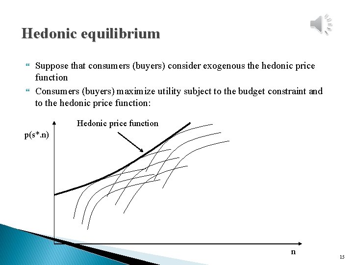
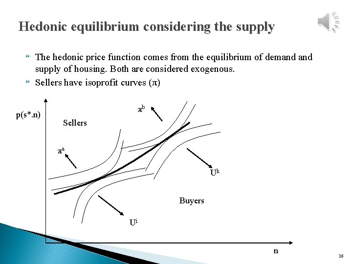
Hedonic equilibrium Suppose that consumers (buyers) consider exogenous the hedonic price function Consumers (buyers) maximize utility subject to the budget constraint and to the hedonic price function: Hedonic price function p(s*. n) n 15

Hedonic equilibrium considering the supply The hedonic price function comes from the equilibrium of demand supply of housing. Both are considered exogenous. Sellers have isoprofit curves (π) p(s*. n) πb Sellers πa Uk Buyers Ui n 16

Marginal Willingness To Pay The main characteristic of the model is that buyers and sellers are efficiently matched along the hedonic price function At any point along the hedonic price function, buyers marginal willingness to pay (and sellers willingness to accept) for a change in n is given by the derivative of the hedonic price function with respect to n. This implicit price changes with n if the hedonic price function is non linear. The model can be generalized to the case where we consider several characteristics of residential properties and of the area where houses are located: p(x 1, x 2, …xk) 17