Status update on ongoing studies M Schenk for

Status update on ongoing studies M. Schenk for EPFL PACMAN team EPFL & CERN, Switzerland Acknowledgements M. Giovannozzi, A. Mereghetti, B. Salvachua, M. Solfaroli, R. Steerenberg, J. Wenninger PACMAN Project Meeting

Overview Three parts 1. LHC: beam lifetime / losses and emittance surrogate model 2. SPS: electro-static septum alignment 3. PS: injection bump optimization 2 02. 12. 2019

LHC: surrogate model for beam lifetimes and emittances L. Coyle, E. Krymova, G. Obozinski, A. Pentina, T. Pieloni, M. Schenk EPFL & CERN, Switzerland PACMAN Project Meeting

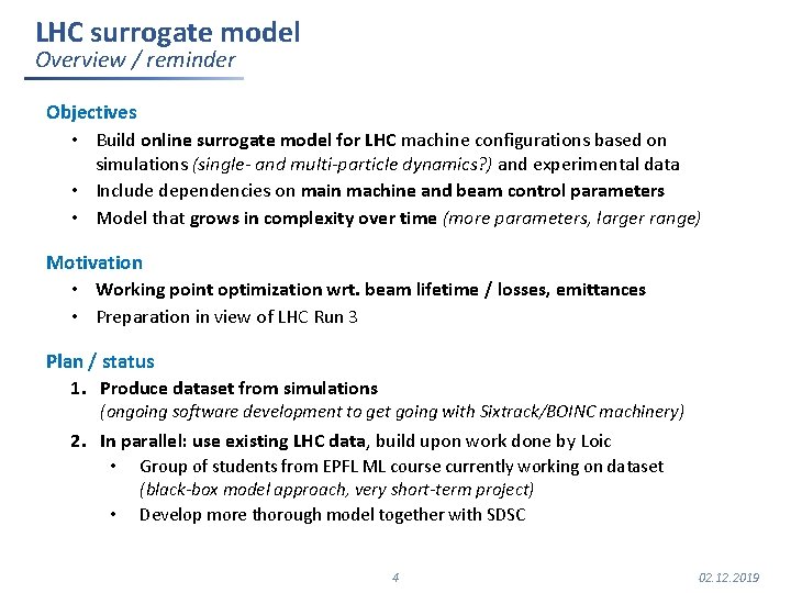
LHC surrogate model Overview / reminder Objectives • Build online surrogate model for LHC machine configurations based on simulations (single- and multi-particle dynamics? ) and experimental data • Include dependencies on main machine and beam control parameters • Model that grows in complexity over time (more parameters, larger range) Motivation • Working point optimization wrt. beam lifetime / losses, emittances • Preparation in view of LHC Run 3 Plan / status 1. Produce dataset from simulations (ongoing software development to get going with Sixtrack/BOINC machinery) 2. In parallel: use existing LHC data, build upon work done by Loic • • Group of students from EPFL ML course currently working on dataset (black-box model approach, very short-term project) Develop more thorough model together with SDSC 4 02. 12. 2019

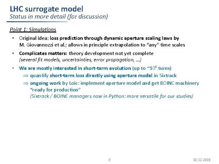
LHC surrogate model Status in more detail (for discussion) Point 1: Simulations • Original idea: loss prediction through dynamic aperture scaling laws by M. Giovannozzi et al. ; allows in principle extrapolation to “any” time scales • Complicates matters: theory development not yet complete (several fit models, uncertainties, error propagation, …) • We are mostly interested in short-term evolution (up to ~106 turns) Þ quantify short-term loss directly using aperture model in Sixtrack Þ ongoing work by Loic: implement aperture model and get BOINC machinery “ready for production” (Sixtrack / BOINC managers now in Python: more versatile for our studies) 5 02. 12. 2019

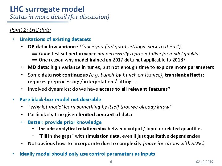
LHC surrogate model Status in more detail (for discussion) Point 2: LHC data • Limitations of existing datasets • OP data: low variance (“once you find good settings, stick to them”) Þ Good test set performance not necessarily representative for model quality Þ One reason why model trained on 2017 data not applicable to 2018? • MD data: high variance in tunes, but not enough time to explore more parameters • Some data not continuous (e. g. bunch-by-bunch emittance), transient effects: requires preprocessing / interpolation / fitting … • Involved dynamics: do we have access to all relevant features? • Pure black-box model not desirable • “Why let model learn something by itself that we already know” • Particularly true given limited amount of data • Better: provide prior knowledge • Include analytical relationships between output / input or related quantities • “Fill in the gaps” with simulation data, even if just qualitative dependencies • Not obvious how to incorporate due to complexity (more iterations with SDSC) • Ideally model should only use control parameters as inputs 6 02. 12. 2019

SPS: electro-static septum alignment M. Schenk�, M. Fraser*, B. Goddard*, S. Hirlaender*�, V. Kain*, T. Pieloni� *CERN & �EPFL, Switzerland �also at University of Malta PACMAN Project Meeting

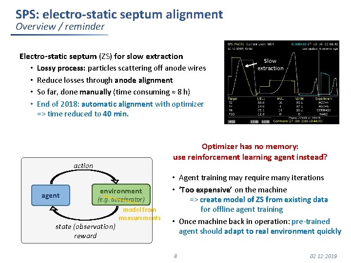
SPS: electro-static septum alignment Overview / reminder Electro-static septum (ZS) for slow extraction • Lossy process: particles scattering off anode wires • Reduce losses through anode alignment • So far, done manually (time consuming ≈ 8 h) • End of 2018: automatic alignment with optimizer Slow extraction => time reduced to 40 min. Optimizer has no memory: use reinforcement learning agent instead? action agent environment (e. g. accelerator) state (observation) reward model from measurements • Agent training may require many iterations • ‘Too expensive’ on the machine => create model of ZS from existing data for offline agent training • Once machine back in operation: pre-trained agent should adapt to real environment quickly 8 02. 12. 2019

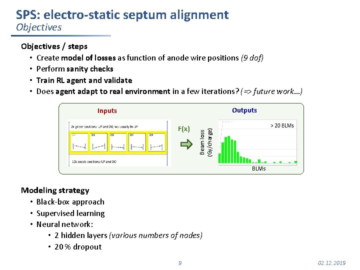
SPS: electro-static septum alignment Objectives / steps • Create model of losses as function of anode wire positions (9 dof) • Perform sanity checks • Train RL agent and validate • Does agent adapt to real environment in a few iterations? (=> future work…) Outputs F(x) Beam loss (Gy/charge) Inputs BLMs Modeling strategy • Black-box approach • Supervised learning • Neural network: • 2 hidden layers (various numbers of nodes) • 20 % dropout 9 02. 12. 2019

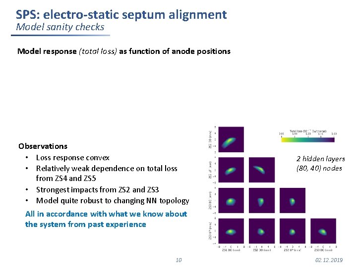
SPS: electro-static septum alignment Model sanity checks Model response (total loss) as function of anode positions Observations • Loss response convex • Relatively weak dependence on total loss 2 hidden layers (80, 40) nodes from ZS 4 and ZS 5 • Strongest impacts from ZS 2 and ZS 3 • Model quite robust to changing NN topology All in accordance with what we know about the system from past experience 10 02. 12. 2019

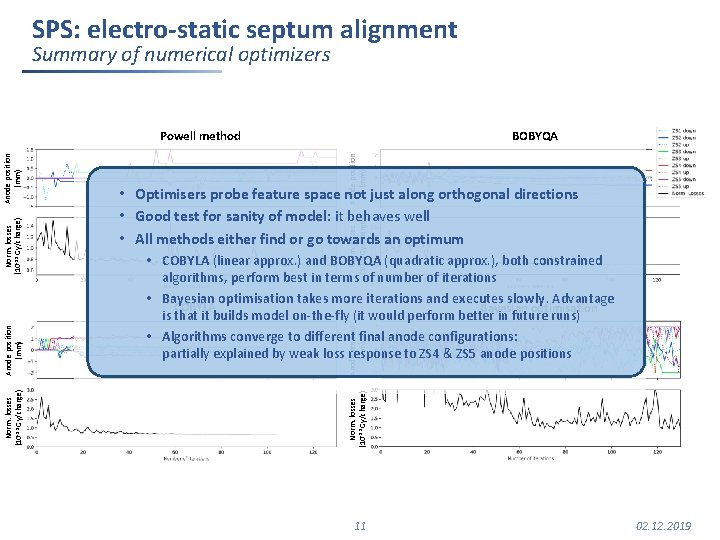
SPS: electro-static septum alignment Summary of numerical optimizers Anode position (mm) BOBYQA Norm. losses (10 -13 Gy/charge) • Optimisers probe feature space not just along orthogonal directions • Good test for sanity of model: it behaves well • All methods either find or go towards an optimum Anode position (mm) • COBYLA (linear approx. ) and BOBYQA (quadratic approx. ), both constrained algorithms, perform best in terms of number of iterations • Bayesian optimisation takes more iterations and executes slowly. Advantage COBYLA Bayesian optimisation is that it builds model on-the-fly (it would perform better in future runs) • Algorithms converge to different final anode configurations: partially explained by weak loss response to ZS 4 & ZS 5 anode positions Norm. losses (10 -13 Gy/charge) Anode position (mm) Powell method 11 02. 12. 2019

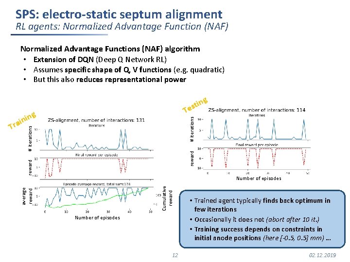
SPS: electro-static septum alignment RL agents: Normalized Advantage Function (NAF) Normalized Advantage Functions (NAF) algorithm • Extension of DQN (Deep Q Network RL) • Assumes specific shape of Q, V functions (e. g. quadratic) • But this also reduces representational power g T # iterations g nin reward # iterations i Tra in est average reward Cumulative reward Number of episodes 12 • Trained agent typically finds back optimum in few iterations • Occasionally it does not (abort after 10 it. ) • Training success depends on constraints in initial anode positions (here [-0. 5, 0. 5] mm) … 02. 12. 2019

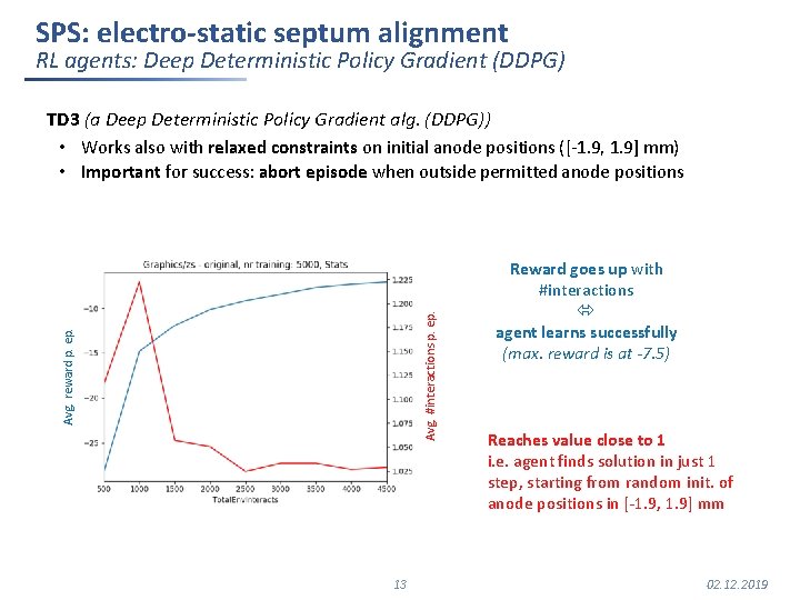
SPS: electro-static septum alignment RL agents: Deep Deterministic Policy Gradient (DDPG) Avg. reward p. ep. Avg. #interactions p. ep. TD 3 (a Deep Deterministic Policy Gradient alg. (DDPG)) • Works also with relaxed constraints on initial anode positions ([-1. 9, 1. 9] mm) • Important for success: abort episode when outside permitted anode positions 13 Reward goes up with #interactions agent learns successfully (max. reward is at -7. 5) Reaches value close to 1 i. e. agent finds solution in just 1 step, starting from random init. of anode positions in [-1. 9, 1. 9] mm 02. 12. 2019

PS: injection bump closure M. Schenk, A. Huschauer EPFL & CERN, Switzerland PACMAN Project Meeting

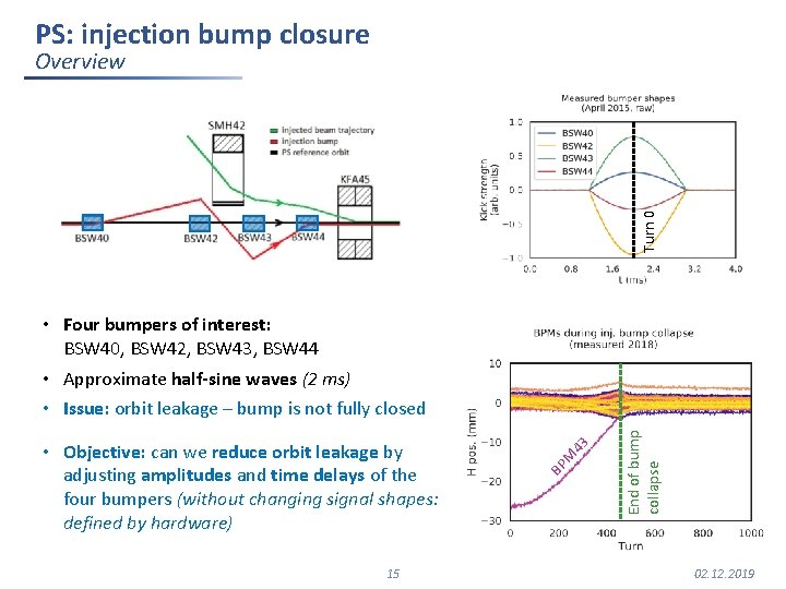
PS: injection bump closure Turn 0 Overview 15 End of bump collapse BP M • Objective: can we reduce orbit leakage by adjusting amplitudes and time delays of the four bumpers (without changing signal shapes: defined by hardware) 43 • Four bumpers of interest: BSW 40, BSW 42, BSW 43, BSW 44 • Approximate half-sine waves (2 ms) • Issue: orbit leakage – bump is not fully closed 02. 12. 2019

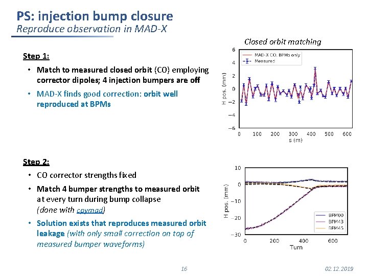
PS: injection bump closure Reproduce observation in MAD-X Closed orbit matching Step 1: • Match to measured closed orbit (CO) employing corrector dipoles; 4 injection bumpers are off • MAD-X finds good correction: orbit well reproduced at BPMs Step 2: • CO corrector strengths fixed • Match 4 bumper strengths to measured orbit at every turn during bump collapse (done with cpymad) • Solution exists that reproduces measured orbit leakage (with only small correction on top of measured bumper waveforms) 16 02. 12. 2019

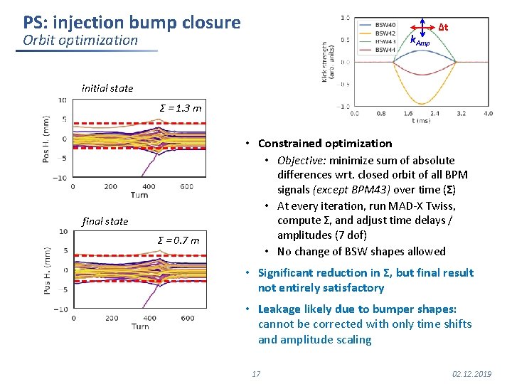
PS: injection bump closure Orbit optimization k. Amp Δt initial state Σ = 1. 3 m • Constrained optimization • Objective: minimize sum of absolute differences wrt. closed orbit of all BPM signals (except BPM 43) over time (Σ) • At every iteration, run MAD-X Twiss, compute Σ, and adjust time delays / amplitudes (7 dof) • No change of BSW shapes allowed final state Σ = 0. 7 m • Significant reduction in Σ, but final result not entirely satisfactory • Leakage likely due to bumper shapes: cannot be corrected with only time shifts and amplitude scaling 17 02. 12. 2019

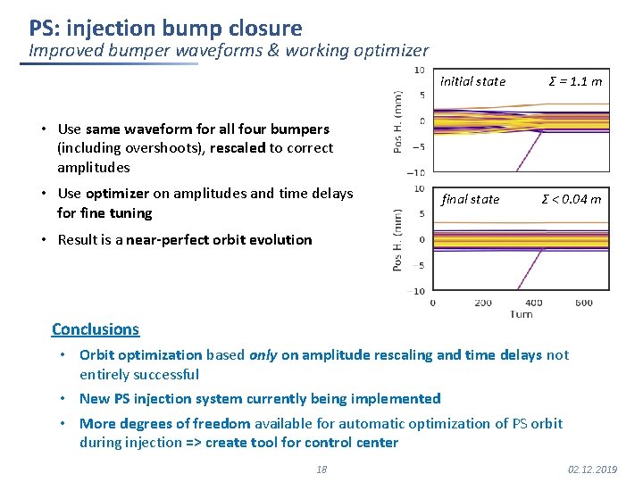
PS: injection bump closure Improved bumper waveforms & working optimizer initial state Σ = 1. 1 m final state Σ < 0. 04 m • Use same waveform for all four bumpers (including overshoots), rescaled to correct amplitudes • Use optimizer on amplitudes and time delays for fine tuning • Result is a near-perfect orbit evolution Conclusions • Orbit optimization based only on amplitude rescaling and time delays not entirely successful • New PS injection system currently being implemented • More degrees of freedom available for automatic optimization of PS orbit during injection => create tool for control center 18 02. 12. 2019