Spatial Classification and Prediction Zhe Jiang zjiangcs ua

Spatial Classification and Prediction Zhe Jiang zjiang@cs. ua. edu 1

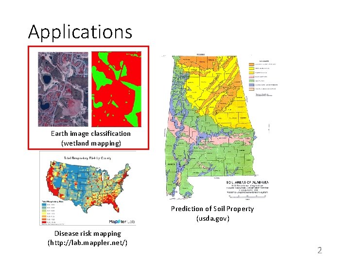
Applications Earth image classification (wetland mapping) Prediction of Soil Property (usda. gov) Disease risk mapping (http: //lab. mappler. net/) 2

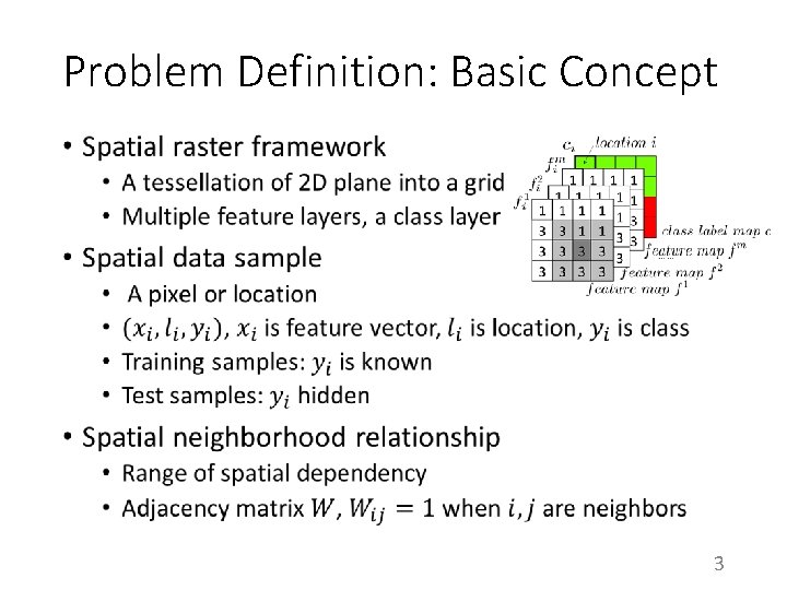
Problem Definition: Basic Concept • 3

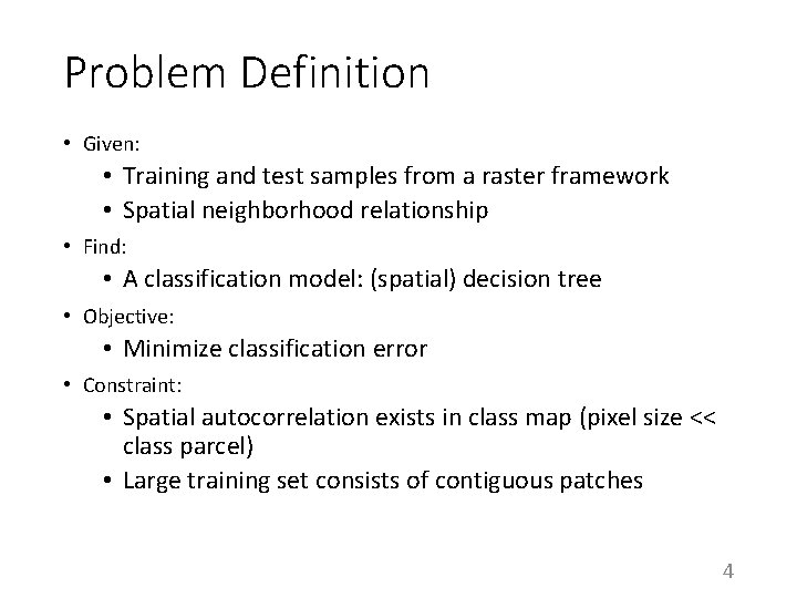
Problem Definition • Given: • Training and test samples from a raster framework • Spatial neighborhood relationship • Find: • A classification model: (spatial) decision tree • Objective: • Minimize classification error • Constraint: • Spatial autocorrelation exists in class map (pixel size << class parcel) • Large training set consists of contiguous patches 4

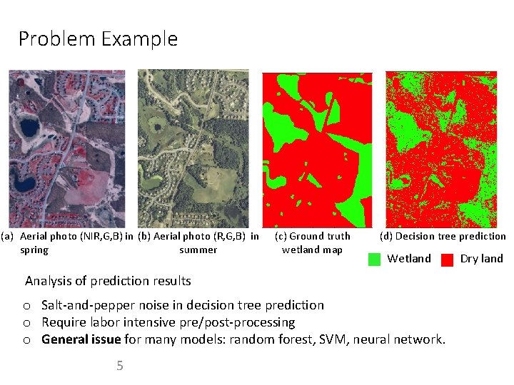
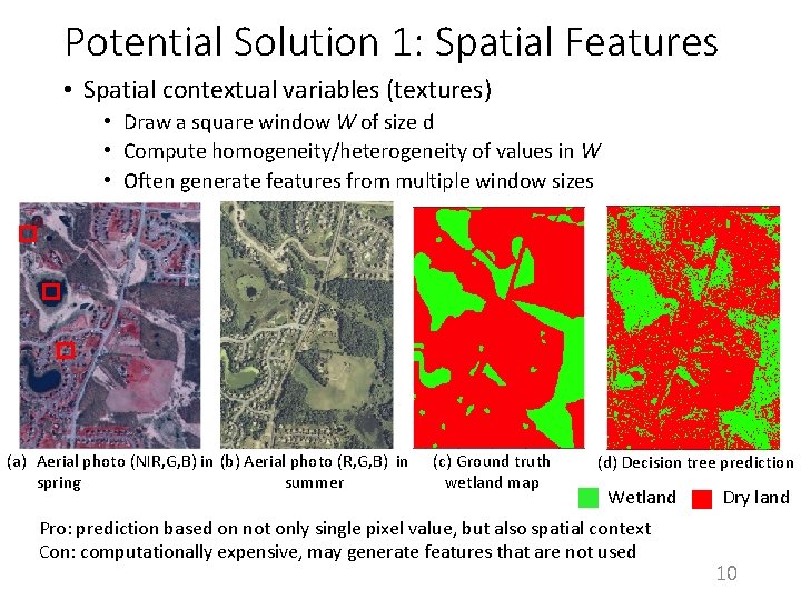
Problem Example (a) Aerial photo (NIR, G, B) in (b) Aerial photo (R, G, B) in spring summer (c) Ground truth wetland map (d) Decision tree prediction Wetland Analysis of prediction results o Salt-and-pepper noise in decision tree prediction o Require labor intensive pre/post-processing o General issue for many models: random forest, SVM, neural network. 5 Dry land

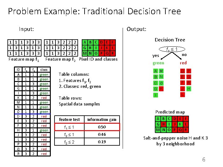
Problem Example: Traditional Decision Tree Input: 1 1 1 3 3 3 1 3 1 1 1 3 3 3 Feature map f 1 ID A B G C G H D M EI N KF M G D N H E O FI DJ K E FL M H P Q NJ O RL C P QI O R f 1 1 3 1 3 1 3 1 3 f 2 1 1 1 3 2 1 3 1 2 2 1 2 3 2 2 1 1 2 3 2 3 2 Output: 1 1 3 2 2 2 A B C D E F G H I J K L M N O P Q R Feature map f 2 Pixel ID and classes class green red green red green red green red Table columns: 1. Features f 1, f 2 2. Classes: red, green Table rows: Spatial data samples Decision Tree yes green f 1 ≤ 1 no red A M B N D P C O F R G K J H I L E Q Predicted map feature test information gain f 1 ≤ 1 0. 50 f 2 ≤ 1 0. 46 f 2 ≤ 2 0. 19 A B C D E F G H I J K L M N O P Q R Salt-and-pepper noise H and K 3 by 3 neighborhood 6

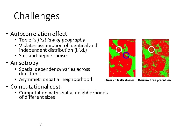
Challenges • Autocorrelation effect • Tobler’s first law of geography • Violates assumption of identical and independent distribution (i. i. d. ) • Salt-and-pepper noise • Anisotropy • Spatial dependency varies across directions • Asymmetric spatial neighborhood • Computational cost Ground truth classes • Computation with spatial neighborhoods of different sizes 7 Decision tree prediction

Potential Solutions • Spatial features • Median filter • Spatial contextual variable (texture) • Focal tree node test • Modify greedy heuristic • Spatial entropy or information gain 8

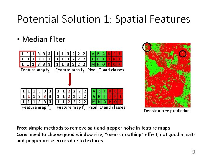
Potential Solution 1: Spatial Features • Median filter 1 1 1 3 3 3 1 3 1 1 1 3 3 3 Feature map f 1 1 3 3 3 1 1 1 3 3 3 Feature map f 1 1 1 3 2 2 2 A B C D E F G H I J K L M N O P Q R 1 1 2 2 2 2 1 1 2 2 A B C D E F G H I J K L M N O P Q R Feature map f 2 Pixel ID and classes Decision tree prediction Pros: simple methods to remove salt-and-pepper noise in feature maps Cons: need to choose good window size; “over-smoothing” effect; not good at saltand-pepper noise errors due to textures 9

Potential Solution 1: Spatial Features • Spatial contextual variables (textures) • Draw a square window W of size d • Compute homogeneity/heterogeneity of values in W • Often generate features from multiple window sizes (a) Aerial photo (NIR, G, B) in (b) Aerial photo (R, G, B) in spring summer (c) Ground truth wetland map (d) Decision tree prediction Wetland Pro: prediction based on not only single pixel value, but also spatial context Con: computationally expensive, may generate features that are not used Dry land 10

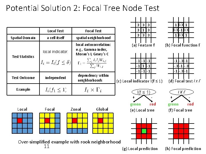
Potential Solution 2: Focal Tree Node Test Spatial Domain Local Test Focal Test a cell itself spatial neighborhood local indicator: Test Statistics Test Outcome independent 3 3 1 3 3 (a) Feature f local autocorrelation: e. g. , Gamma index, Moran’s I, Geary’s C dependency within neighborhoods -1 -1 -1 (c) Local indicator I(f ≤ 1) Example Local I(f ≤ 1) Focal Zonal Global + green red (e) Local tree 1 0. 3 -1 0. 3 1 (b) Focal function Γ -1 -. 3 -1 (d) Focal test I X Γ IXΓ + green red (f) Focal tree Over-simplified example with rook neighborhood 11 (g) Local prediction (h) Focal prediction

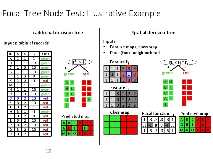
Focal Tree Node Test: Illustrative Example Traditional decision tree Spatial decision tree Inputs: • Feature maps, class map • Rook (four) neighborhood Inputs: table of records ID A B C G D EI KF M G N H OI DJ K E FL M H NJ O L P Q R f 1 1 3 1 3 1 3 3 3 3 f 2 1 1 3 2 1 2 3 2 1 1 3 2 2 2 1 1 2 3 2 2 Γ 1 1 0. 3 0 -1 1 0. 3 1 -1 0 0. 3 1 class green red green green red red green red red 12 I(f 1 ≤ 1) - + green red A M D P B N C O G K E Q F R J H L I Predicted map A B C D E F G H I J K L M N O P Q R Feature f 1 1 3 3 3 1 3 1 1 1 3 3 3 Feature f 2 1 1 3 2 2 2 Class map I(f 1 ≤ 1) * Γ 1 + green red A M D P B N C O G H E Q F R J K L I Focal function Γ 1 1. 3. 3 1. 3 -1 0 0 -1. 3. 3 1 Predicted map A B C D E F G H I J K L M N O P Q R

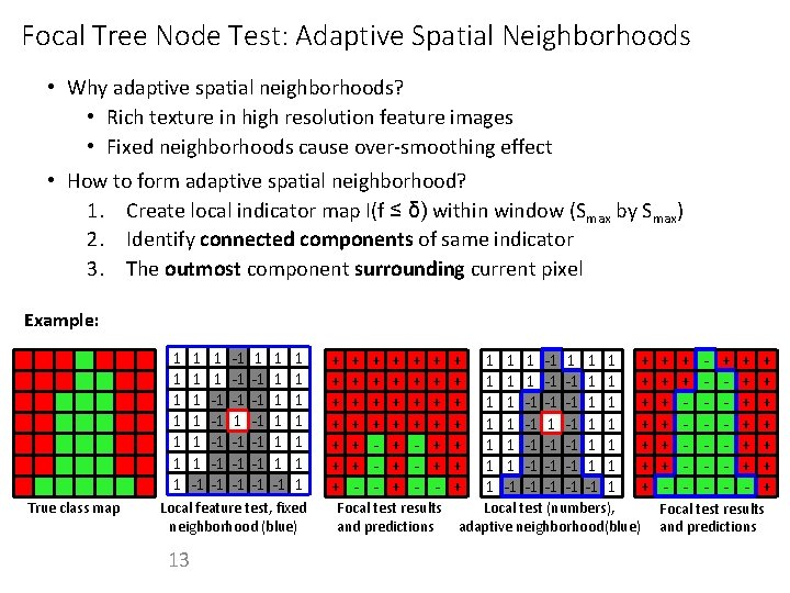
Focal Tree Node Test: Adaptive Spatial Neighborhoods • Why adaptive spatial neighborhoods? • Rich texture in high resolution feature images • Fixed neighborhoods cause over-smoothing effect • How to form adaptive spatial neighborhood? 1. Create local indicator map I(f ≤ δ) within window (Smax by Smax) 2. Identify connected components of same indicator 3. The outmost component surrounding current pixel Example: 1 1 1 1 True class map 1 1 1 -1 -1 -1 -1 -1 -1 1 1 1 1 Local feature test, fixed neighborhood (blue) 13 + + + + + + + - + + + + 1 1 1 1 -1 1 1 -1 -1 -1 -1 -1 -1 1 1 1 + + + + Focal test results Local test (numbers), and predictions adaptive neighborhood(blue) + + + - - + + + + Focal test results and predictions

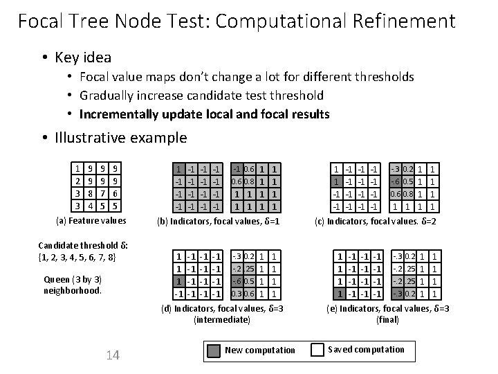
Focal Tree Node Test: Computational Refinement • Key idea • Focal value maps don’t change a lot for different thresholds • Gradually increase candidate test threshold • Incrementally update local and focal results • Illustrative example 1 2 3 3 9 9 8 4 9 9 7 5 9 9 6 5 (a) Feature values Candidate threshold δ: {1, 2, 3, 4, 5, 6, 7, 8} Queen (3 by 3) neighborhood. 14 1 -1 -1 -1 -1 0. 6 1 1 0. 6 0. 8 1 1 1 1 1 (b) Indicators, focal values, δ=1 1 -1 -. 3 0. 2 1 1 1 -1 -. 2. 25 1 1 1 -1 -. 6 0. 5 1 1 -1 -1 0. 3 0. 6 1 1 (d) Indicators, focal values, δ=3 (intermediate) New computation 1 1 -1 -1 -1 -1 1 1 1 -. 3 0. 2 -. 6 0. 5 0. 6 0. 8 1 1 (c) Indicators, focal values. δ=2 1 -1 -. 3 0. 2 1 1 1 -1 -1 -1 -. 2. 25 1 1 1 -1 -. 3 0. 2 1 1 (e) Indicators, focal values, δ=3 (final) Saved computation

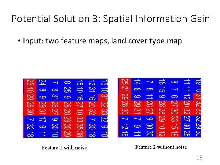
Potential Solution 3: Spatial Information Gain • Input: two feature maps, land cover type map Feature 1 with noise Feature 2 without noise 15

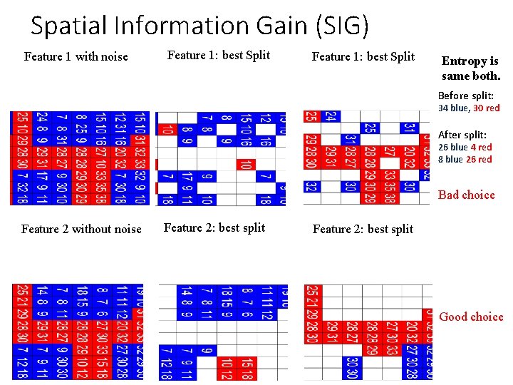
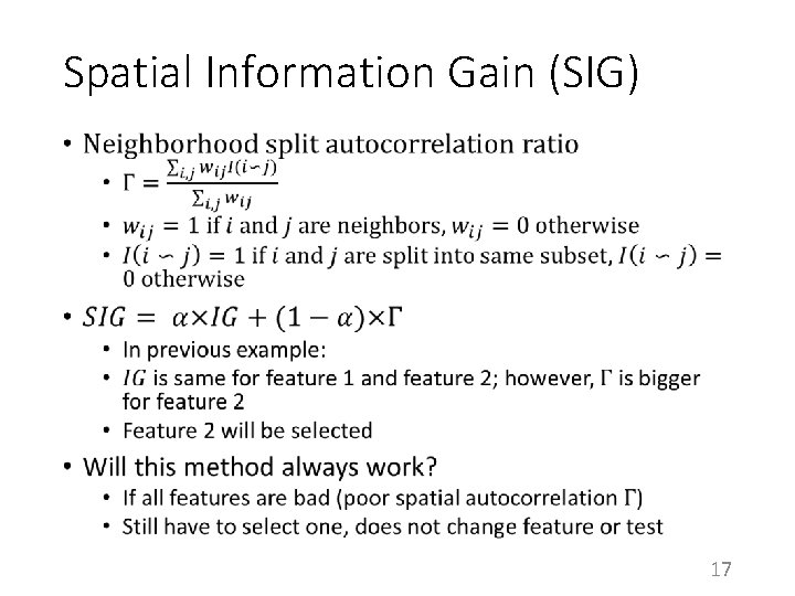
Spatial Information Gain (SIG) Feature 1 with noise Feature 1: best Split Entropy is same both. Before split: 34 blue, 30 red After split: 26 blue 4 red 8 blue 26 red Bad choice Feature 2 without noise Feature 2: best split Good choice

Spatial Information Gain (SIG) • 17

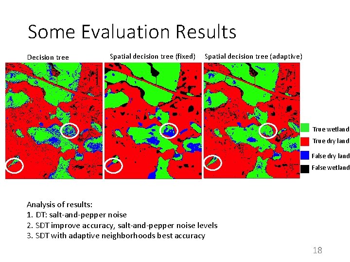
Some Evaluation Results Decision tree Spatial decision tree (fixed) Spatial decision tree (adaptive) True wetland True dry land False wetland Analysis of results: 1. DT: salt-and-pepper noise 2. SDT improve accuracy, salt-and-pepper noise levels 3. SDT with adaptive neighborhoods best accuracy 18

Summary • Three approaches to enhance decision trees for spatial classification • Spatial features • Spatial tree node test formula • Spatial greedy heuristic • Focal-test in tree nodes is effective, but additional challenges remain 19

References: [1]: Jiang Z, Shekhar S, Zhou X, Knight J, Corcoran J. Focal-test-based spatial decision tree learning. IEEE Transactions on Knowledge and Data Engineering. 2015 Jun 1; 27(6): 1547 -59. [2]: Jiang Z, Shekhar S, Mohan P, Knight J, Corcoran J. Learning spatial decision tree for geographical classification: a summary of results. In. Proceedings of the 20 th International Conference on Advances in Geographic Information Systems 2012 Nov 6 (pp. 390 -393). ACM. 20