Trajectory Clustering Tianxiao Jiang Biomedical Engineering Department University

Trajectory Clustering Tianxiao Jiang, Biomedical Engineering Department, University of Houston

Visual aided approach • Automatic method may discover movement patterns that are interesting but trivial. • Visual analytics can control the computational process.

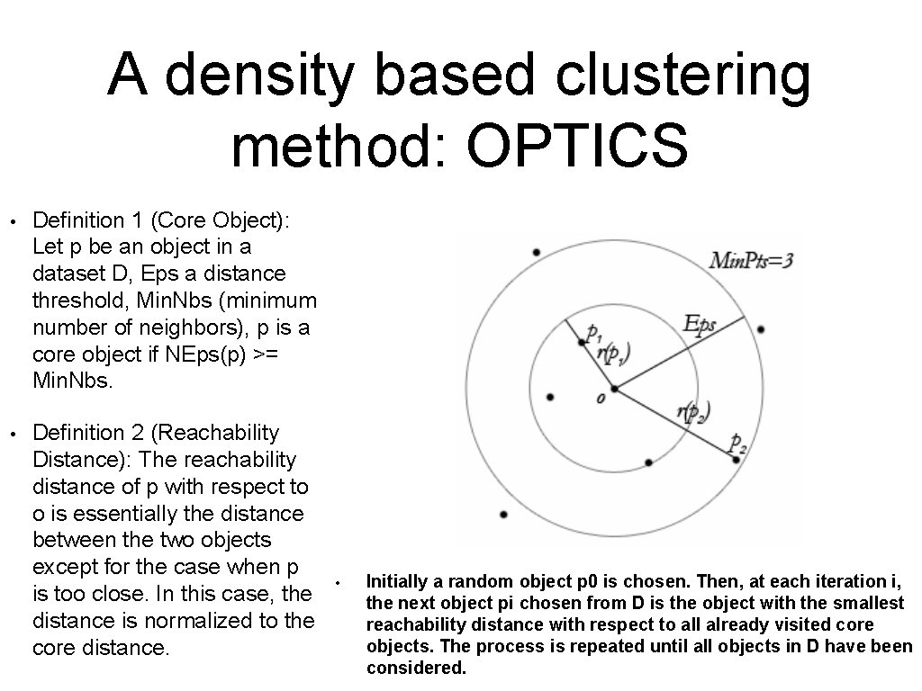
A density based clustering method: OPTICS • Definition 1 (Core Object): Let p be an object in a dataset D, Eps a distance threshold, Min. Nbs (minimum number of neighbors), p is a core object if NEps(p) >= Min. Nbs. • Definition 2 (Reachability Distance): The reachability distance of p with respect to o is essentially the distance between the two objects except for the case when p is too close. In this case, the distance is normalized to the core distance. • Initially a random object p 0 is chosen. Then, at each iteration i, the next object pi chosen from D is the object with the smallest reachability distance with respect to all already visited core objects. The process is repeated until all objects in D have been considered.

Progressive Clustering • A large value Min. Nbs (decide core object) is applied • Analyst play with parameters (Eps, Min. Nbs) until getting a few clusters that are spatially coherent and well interpretable • After examining, describing, and explaining the most significant clusters, the analyst excludes their members from the further analysis and applies clustering with smaller Min. Nbs to the remaining data • Repeat the process (Go to the second step)

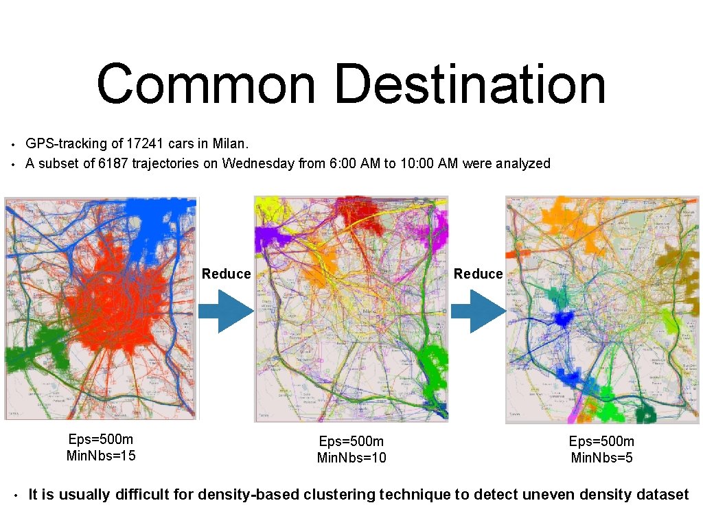
Common Destination • • GPS-tracking of 17241 cars in Milan. A subset of 6187 trajectories on Wednesday from 6: 00 AM to 10: 00 AM were analyzed Reduce Eps=500 m Min. Nbs=15 • Reduce Eps=500 m Min. Nbs=10 Eps=500 m Min. Nbs=5 It is usually difficult for density-based clustering technique to detect uneven density dataset

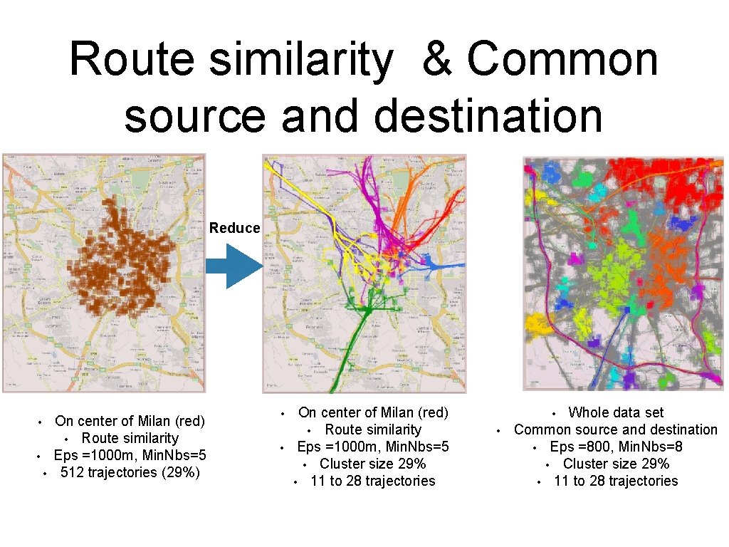
Route similarity & Common source and destination Reduce • • • On center of Milan (red) • Route similarity Eps =1000 m, Min. Nbs=5 512 trajectories (29%) • • On center of Milan (red) • Route similarity Eps =1000 m, Min. Nbs=5 • Cluster size 29% • 11 to 28 trajectories Whole data set Common source and destination • Eps =800, Min. Nbs=8 • Cluster size 29% • 11 to 28 trajectories • •

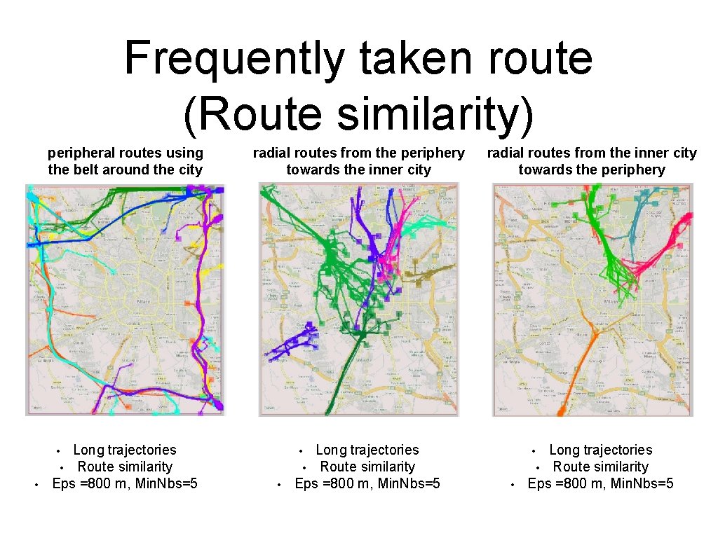
Frequently taken route (Route similarity) peripheral routes using the belt around the city Long trajectories • Route similarity Eps =800 m, Min. Nbs=5 radial routes from the periphery towards the inner city • • Long trajectories • Route similarity Eps =800 m, Min. Nbs=5 radial routes from the inner city towards the periphery • • Long trajectories • Route similarity Eps =800 m, Min. Nbs=5 • •

Micro-clustering • • • Traditional trajectory clustering algorithm group similar trajectory as a whole, sometimes it can miss common sub-trajectory. Trajectory might have different lengths Discovering common sub-trajectory is very useful in some applications.

Micro clustering 1 • Represent trajectory as piece-wise segments (possibly with missing intervals) • Find a maximal segment where all trajectories are pair-wise close to each other • The similarity of trajectories is based on the time length of close segments

Micro clustering 2 • Segments of different trajectories within a given rectangle are grouped together if they occur in similar time intervals • Determine the maximal group size and temporal dimension within the threshold rectangle

Micro clustering 3 A Partition-and-Group Framework • Partition trajectory into sub-trajectories using minimum description length (MDL) principle • Group similar segments using a density based clustering algorithm

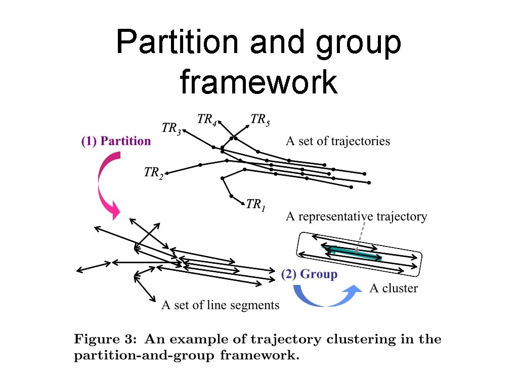
Partition and group framework

Q: Why not prune the ‘useless’ part of the trajectory so that we can use traditional clustering algorithm on the ‘interesting’ part of the trajectory ? • It is tricky to determine which part is ‘useless’ and which part is ‘important’. • ‘Pruning’ forbids us from discovering unexpected clustering results.

Q: Why density-based clustering ? • Trajectory is often of arbitrary shapes and noisy • Density-based clustering methods [2, 6] are the most suitable for line segments because they can discover clusters of arbitrary shape and can filter out noises [11].

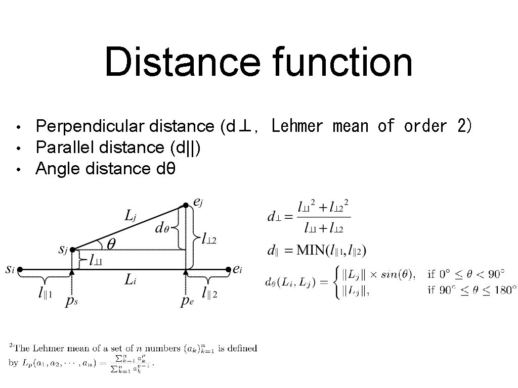
Distance function • • • Perpendicular distance (d⊥, Lehmer mean of order 2) Parallel distance (d||) Angle distance dθ

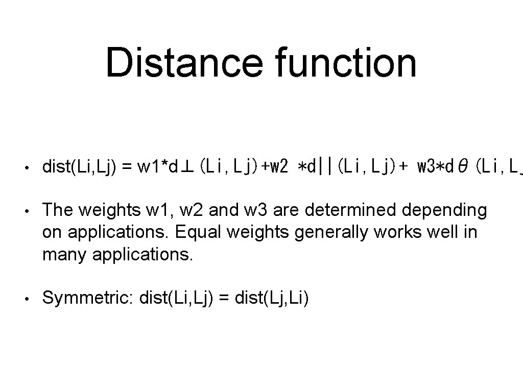
Distance function • dist(Li, Lj) = w 1*d⊥(Li, Lj)+w 2 *d||(Li, Lj)+ w 3*dθ(Li, Lj • The weights w 1, w 2 and w 3 are determined depending on applications. Equal weights generally works well in many applications. • Symmetric: dist(Li, Lj) = dist(Lj, Li)

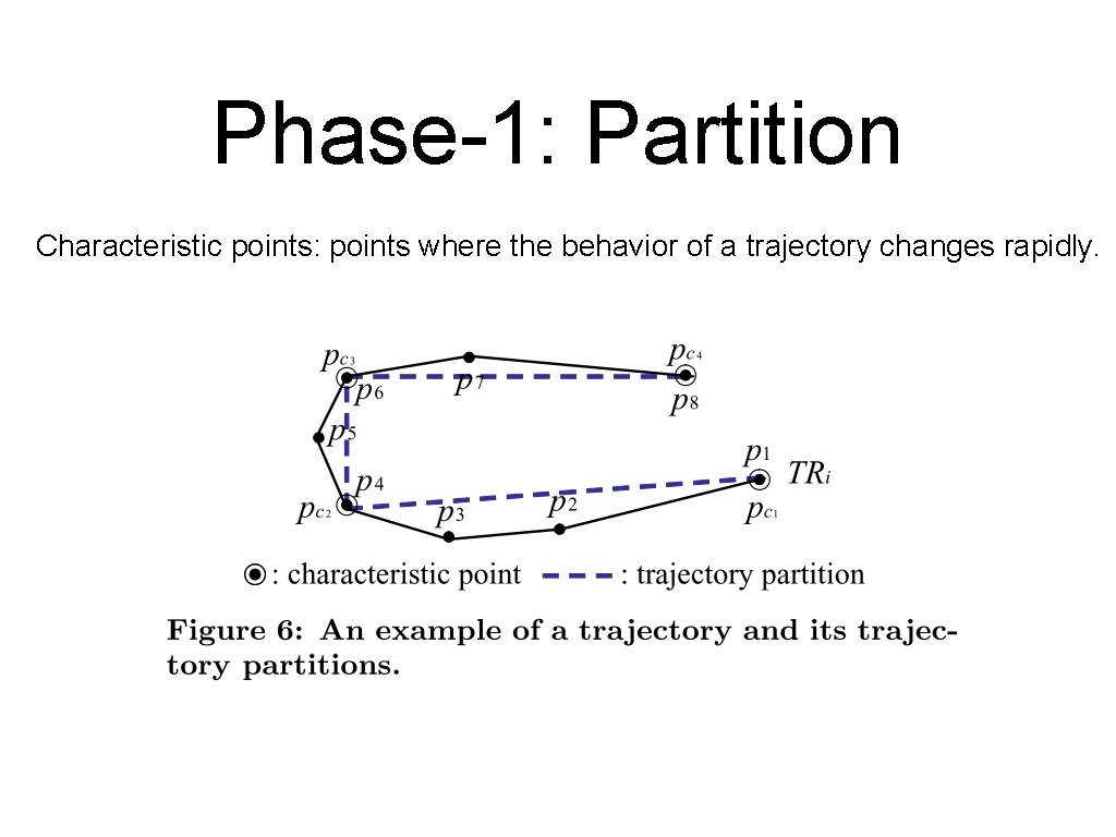
Phase-1: Partition Characteristic points: points where the behavior of a trajectory changes rapidly.

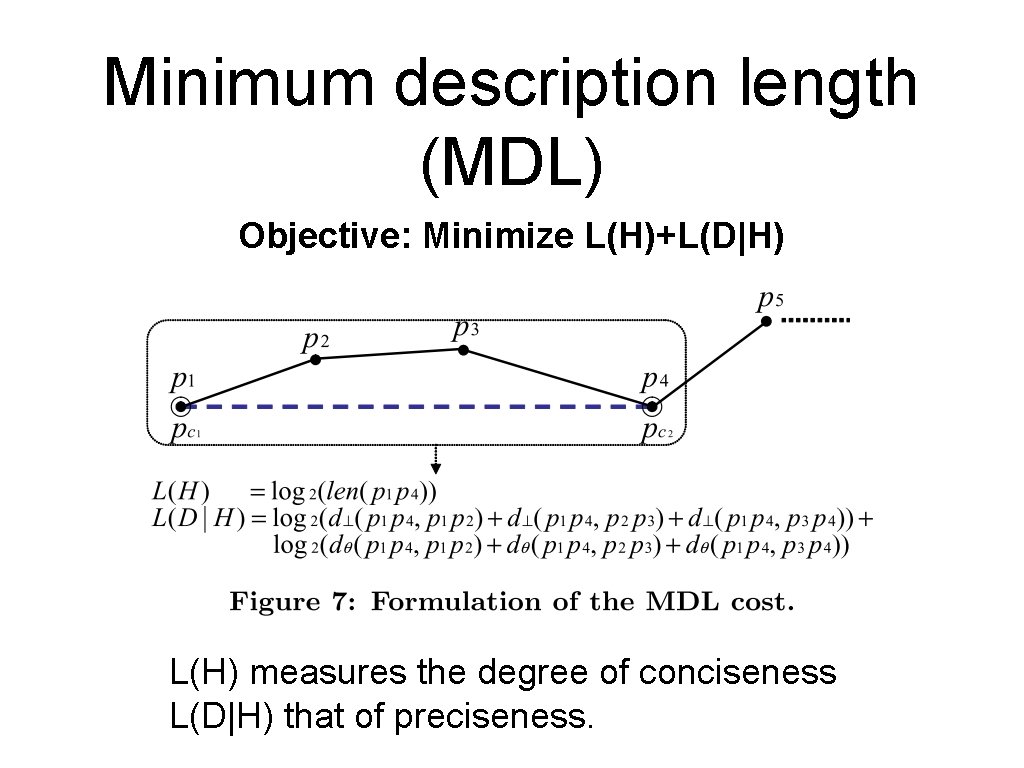
Minimum description length (MDL) Objective: Minimize L(H)+L(D|H) L(H) measures the degree of conciseness L(D|H) that of preciseness.

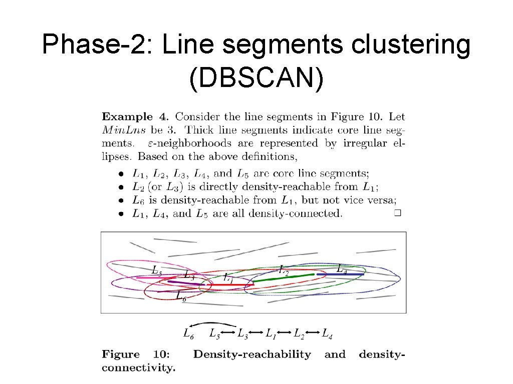
Phase-2: Line segments clustering (DBSCAN)

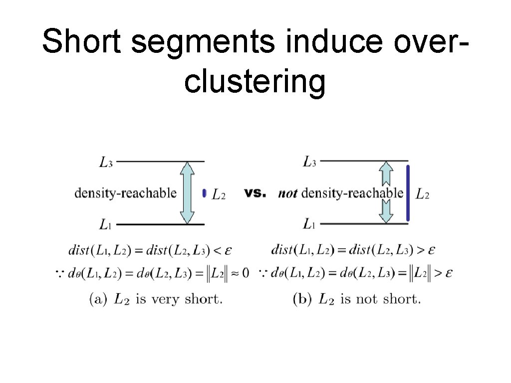
Short segments induce overclustering

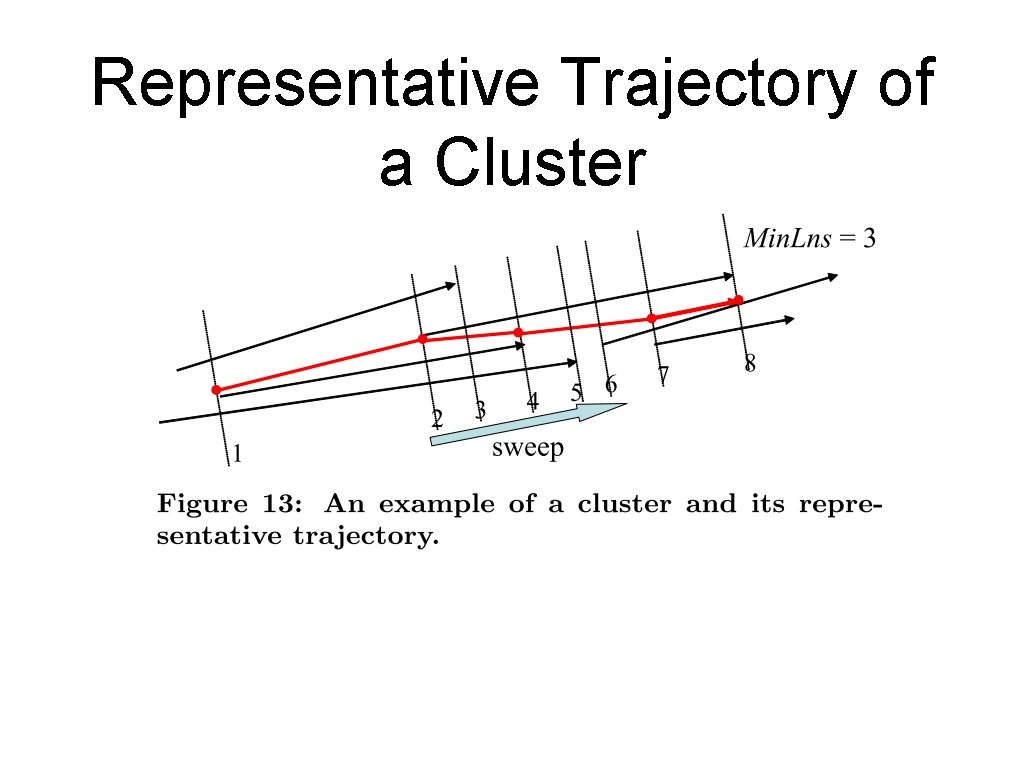
Representative Trajectory of a Cluster

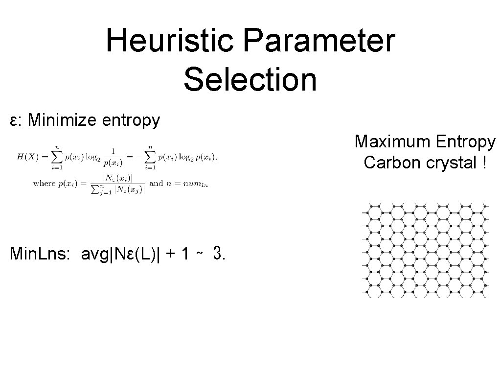
Heuristic Parameter Selection ε: Minimize entropy Maximum Entropy Carbon crystal ! Min. Lns: avg|Nε(L)| + 1 ∼ 3.

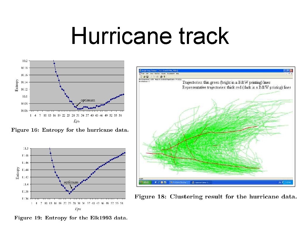
Hurricane track

Flocks and Convoy • Discovering group of objects that move together during a given period of time. For example, migrating animals, flocks of birds or convoys of vehicles • e. g. propose moving clusters to describe the problem of discovery of sequence of clusters in which objects may leave or enter the cluster during some time interval but having the portion of common objects higher than a predefined threshold…

The End