Sketching via Hashing from Heavy Hitters to Compressive

Sketching via Hashing: from Heavy Hitters to Compressive Sensing to Sparse Fourier Transform Piotr Indyk MIT

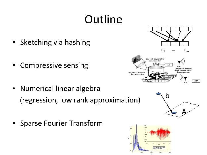
Outline • Sketching via hashing c 1 … cm • Compressive sensing • Numerical linear algebra (regression, low rank approximation) b A • Sparse Fourier Transform

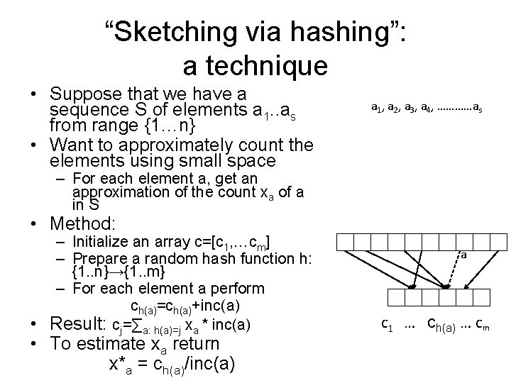
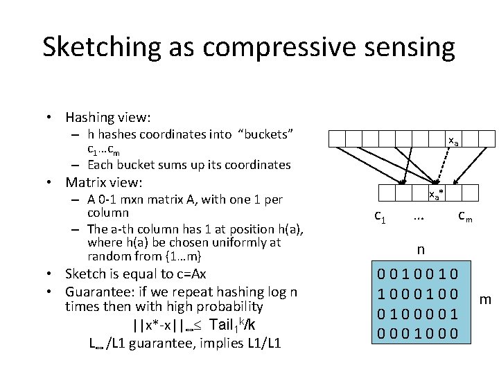
“Sketching via hashing”: a technique • Suppose that we have a sequence S of elements a 1. . as from range {1…n} • Want to approximately count the elements using small space a 1, a 2, a 3, a 4, …………as – For each element a, get an approximation of the count xa of a in S • Method: – Initialize an array c=[c 1, …cm] – Prepare a random hash function h: {1. . n}→{1. . m} – For each element a perform ch(a)=ch(a)+inc(a) • Result: cj=∑a: h(a)=j xa * inc(a) • To estimate xa return x*a = ch(a)/inc(a) a c 1 … ch(a) … cm

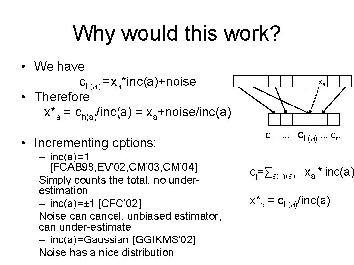
Why would this work? • We have ch(a) =xa*inc(a)+noise • Therefore x*a = ch(a)/inc(a) = xa+noise/inc(a) • Incrementing options: – inc(a)=1 [FCAB 98, EV’ 02, CM’ 03, CM’ 04] Simply counts the total, no underestimation – inc(a)=± 1 [CFC’ 02] Noise cancel, unbiased estimator, can under-estimate – inc(a)=Gaussian [GGIKMS’ 02] Noise has a nice distribution xa c 1 … ch(a) … cm cj=∑a: h(a)=j xa * inc(a) x*a = ch(a)/inc(a)

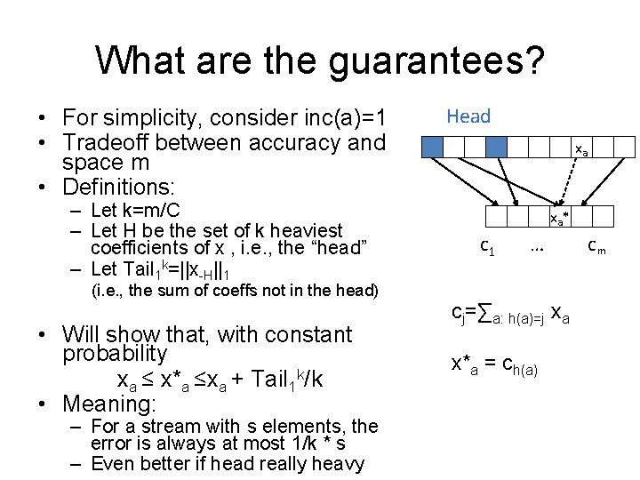
What are the guarantees? • For simplicity, consider inc(a)=1 • Tradeoff between accuracy and space m • Definitions: – Let k=m/C – Let H be the set of k heaviest coefficients of x , i. e. , the “head” – Let Tail 1 k=||x-H||1 (i. e. , the sum of coeffs not in the head) • Will show that, with constant probability xa ≤ x*a ≤xa + Tail 1 k/k • Meaning: – For a stream with s elements, the error is always at most 1/k * s – Even better if head really heavy Head xa xa * c 1 … cm cj=∑a: h(a)=j xa x*a = ch(a)

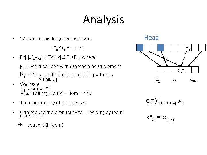
Analysis • We show to get an estimate Head xa x*a ≤xa + Tail / k • • Pr[ |x*a-xa| > Tail/k] ≤ P 1+P 2, where P 1 = Pr[ a collides with (another) head element ] P 2 = Pr[ sum of tail elems colliding with a is > Tail/k ] We have P 1 ≤ k/m =1/C P 2 ≤ (Tail/m)/(Tail/k) = k/m = 1/C • Total probability of failure ≤ 2/C • Can reduce the probability to 1/poly(n) by log n repetitions space O(k log n) xa * c 1 … cm cj=∑a: h(a)=j xa x*a = ch(a)

Compressive sensing

Compressive sensing [Candes-Romberg-Tao, Donoho] • (also: approximation theory, learning Fourier coeffs, finite rate of innovation, …) Setup: – Data/signal in n-dimensional space : x E. g. , x is an 256 x 256 image n=65536 – Goal: compress x into a “measurement” Ax , where A is a m x n “measurement matrix”, m << n • Requirements: – Plan A: want to recover x from Ax • Impossible: underdetermined system of equations – Plan B: want to recover an “approximation” x* of x • Sparsity parameter k • Informally: want to recover largest k coordinates of x • Formally: want x* such that e. g. (L 1/L 1) ||x*-x||1 C minx’ ||x’-x||1 =C Tail 1 k over all x’ that are k-sparse (at most k non-zero entries) • Want: – Good compression (small m=m(k, n)) – Efficient algorithms for encoding and recovery • Why linear compression ? A x = Ax

Applications • Single pixel camera [Wakin, Laska, Duarte, Baron, Sarvotham, Takhar, Kelly, Baraniuk’ 06] • Pooling Experiments [Kainkaryam, Woolf’ 08], [Hassibi et al’ 07], [Dai-Sheikh, Milenkovic, Baraniuk], [Shental-Amir-Zuk’ 09], [Erlich-Shental-Amir. Zuk’ 09], [Kainkaryam, Bruex, Gilbert, Woolf’ 10]…

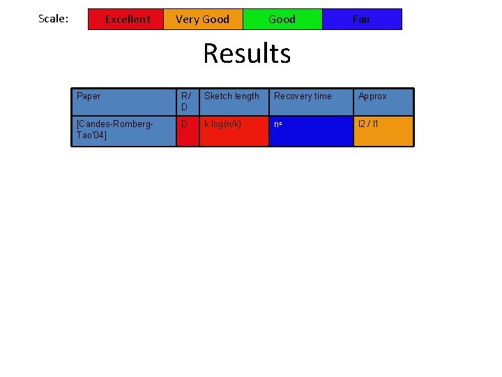
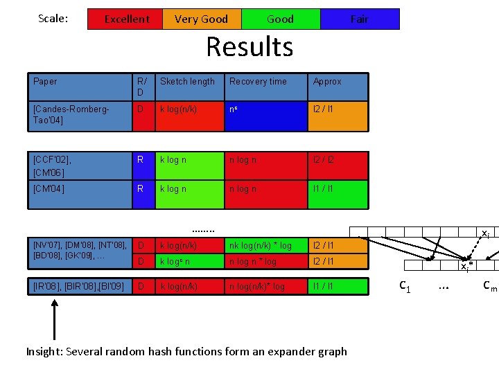
Scale: Excellent Very Good Fair Results Paper R/ D Sketch length Recovery time Approx [Candes-Romberg. Tao’ 04] D k log(n/k) nc l 2 / l 1

Sketching as compressive sensing • Hashing view: – h hashes coordinates into “buckets” c 1…cm – Each bucket sums up its coordinates xa • Matrix view: – A 0 -1 mxn matrix A, with one 1 per column – The a-th column has 1 at position h(a), where h(a) be chosen uniformly at random from {1…m} • Sketch is equal to c=Ax • Guarantee: if we repeat hashing log n times then with high probability ||x*-x||∞ Tail 1 k/k L∞ /L 1 guarantee, implies L 1/L 1 xa * c 1 … cm n 0 0 1 0 1 0 0 m 0 1 0 0 0

Scale: Excellent Very Good Fair Results Paper R/ D Sketch length Recovery time Approx [Candes-Romberg. Tao’ 04] D k log(n/k) nc l 2 / l 1 [CCF’ 02], [CM’ 06] R k log n n log n l 2 / l 2 [CM’ 04] R k log n n log n l 1 / l 1 ……. . [NV’ 07], [DM’ 08], [NT’ 08], [BD’ 08], [GK’ 09], … D k log(n/k) nk log(n/k) * log l 2 / l 1 D k logc n n log n * log l 2 / l 1 [IR’ 08], [BI’ 09] D k log(n/k) n log(n/k)* log l 1 / l 1 Insight: Several random hash functions form an expander graph xi xi * c 1 … cm

Regression

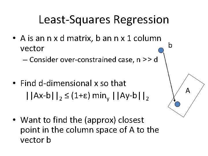
Least-Squares Regression • A is an n x d matrix, b an n x 1 column b vector – Consider over-constrained case, n >> d • Find d-dimensional x so that ||Ax-b||2 ≤ (1+ε) miny ||Ay-b||2 • Want to find the (approx) closest point in the column space of A to the vector b A

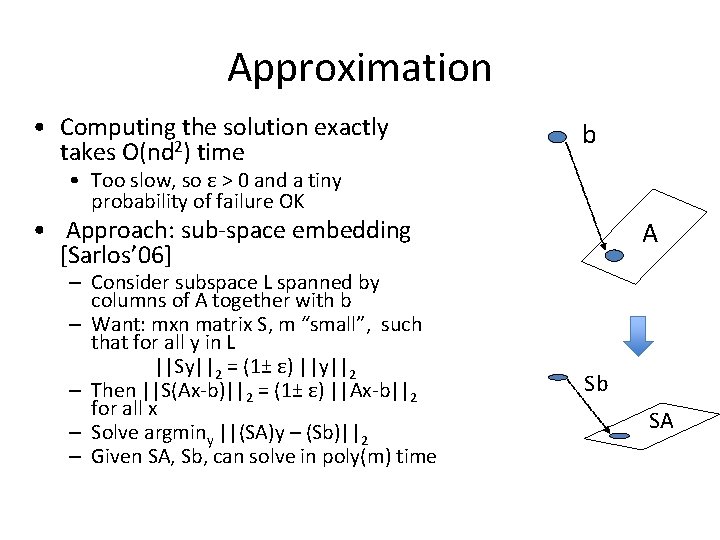
Approximation • Computing the solution exactly takes O(nd 2) time b • Too slow, so ε > 0 and a tiny probability of failure OK • Approach: sub-space embedding [Sarlos’ 06] – Consider subspace L spanned by columns of A together with b – Want: mxn matrix S, m “small”, such that for all y in L ||Sy||2 = (1± ε) ||y||2 – Then ||S(Ax-b)||2 = (1± ε) ||Ax-b||2 for all x – Solve argminy ||(SA)y – (Sb)||2 – Given SA, Sb, can solve in poly(m) time A Sb SA

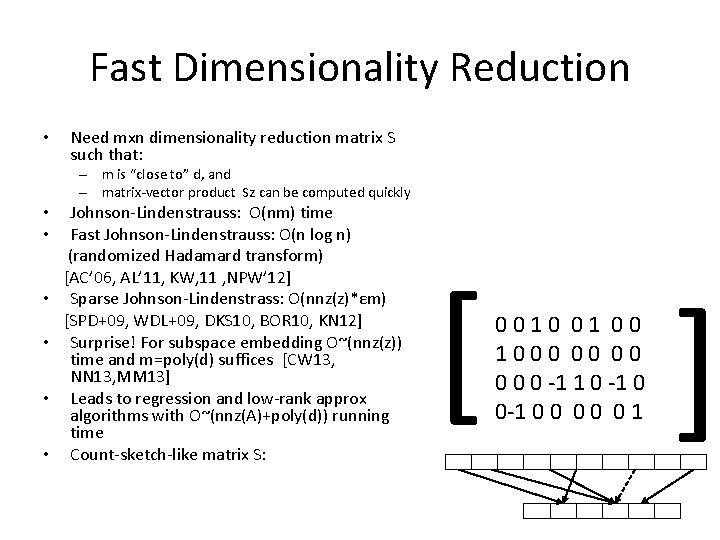
Fast Dimensionality Reduction • Need mxn dimensionality reduction matrix S such that: – m is “close to” d, and – matrix-vector product Sz can be computed quickly • Johnson-Lindenstrauss: O(nm) time • Fast Johnson-Lindenstrauss: O(n log n) (randomized Hadamard transform) [AC’ 06, AL’ 11, KW, 11 , NPW’ 12] • Sparse Johnson-Lindenstrass: O(nnz(z)*εm) [SPD+09, WDL+09, DKS 10, BOR 10, KN 12] • Surprise! For subspace embedding O~(nnz(z)) time and m=poly(d) suffices [CW 13, NN 13, MM 13] • Leads to regression and low-rank approx algorithms with O~(nnz(A)+poly(d)) running time • Count-sketch-like matrix S: [ 0 0 1 0 0 0 0 0 -1 1 0 -1 0 0 0 0 0 1

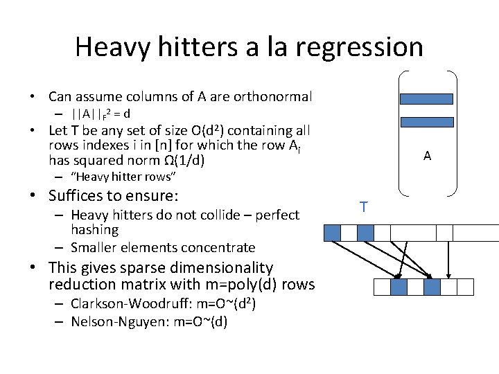
Heavy hitters a la regression • Can assume columns of A are orthonormal – ||A||F 2 = d • Let T be any set of size O(d 2) containing all rows indexes i in [n] for which the row Ai has squared norm Ω(1/d) A – “Heavy hitter rows” • Suffices to ensure: – Heavy hitters do not collide – perfect hashing – Smaller elements concentrate • This gives sparse dimensionality reduction matrix with m=poly(d) rows – Clarkson-Woodruff: m=O~(d 2) – Nelson-Nguyen: m=O~(d) T

Sparse Fourier Transform

Fourier Transform • Discrete Fourier Transform: – Given: a signal x[1…n] – Goal: compute the frequency vector x’ where x’f = Σt xt e-2πi tf/n • Very useful tool: – – Compression (audio, image, video) Data analysis Feature extraction … • See SIGMOD’ 04 tutorial “Indexing and Mining Streams” by C. Faloutsos Sampled Audio Data (Time) DFT of Audio Samples (Frequency)

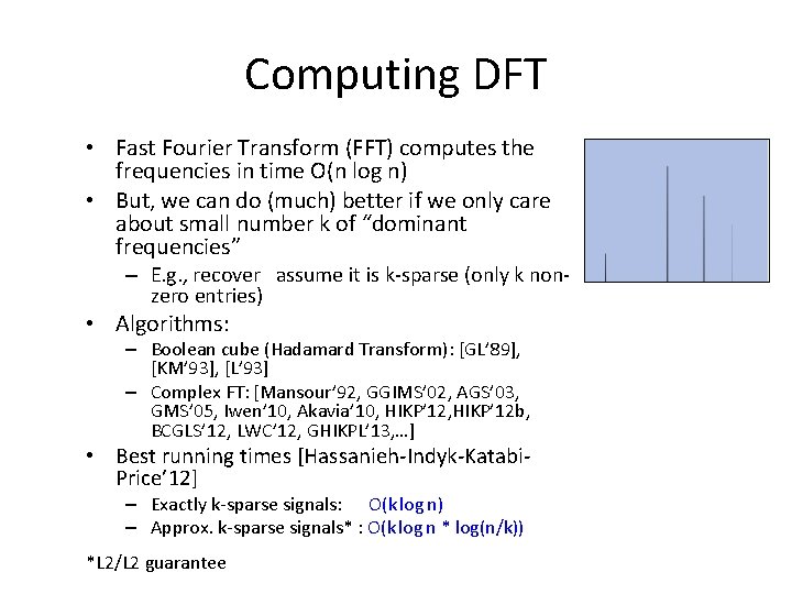
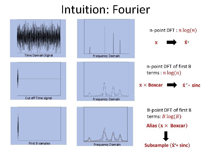
Computing DFT • Fast Fourier Transform (FFT) computes the frequencies in time O(n log n) • But, we can do (much) better if we only care about small number k of “dominant frequencies” – E. g. , recover assume it is k-sparse (only k nonzero entries) • Algorithms: – Boolean cube (Hadamard Transform): [GL’ 89], [KM’ 93], [L’ 93] – Complex FT: [Mansour’ 92, GGIMS’ 02, AGS’ 03, GMS’ 05, Iwen’ 10, Akavia’ 10, HIKP’ 12 b, BCGLS’ 12, LWC’ 12, GHIKPL’ 13, …] • Best running times [Hassanieh-Indyk-Katabi. Price’ 12] – Exactly k-sparse signals: O(k log n) – Approx. k-sparse signals* : O(k log n * log(n/k)) *L 2/L 2 guarantee

Intuition: Fourier Time Domain Signal ‘ Frequency Domain Cut off Time signal ‘ Frequency Domain First B samples Frequency Domain ‘

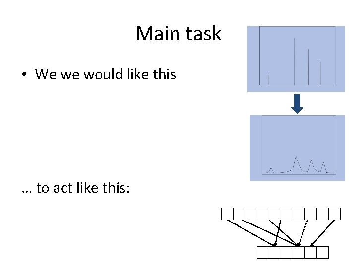
Main task • We we would like this … to act like this:

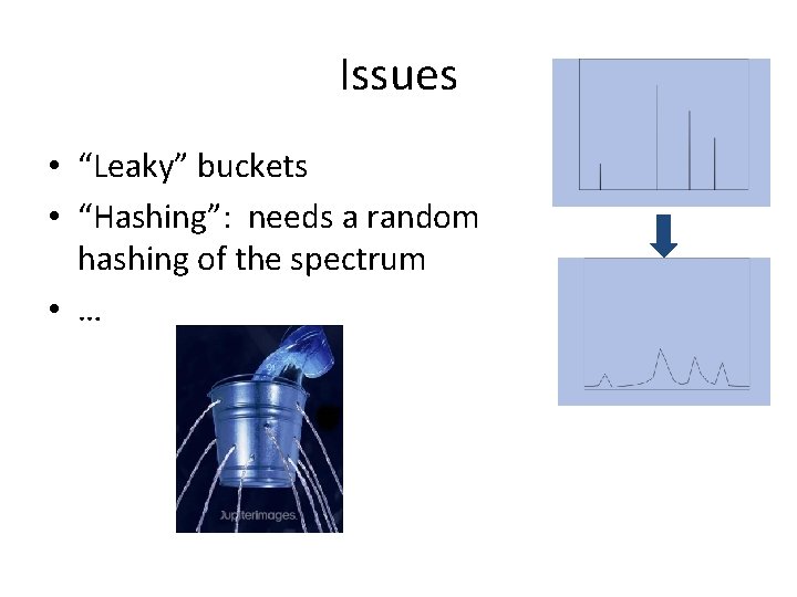
Issues • “Leaky” buckets • “Hashing”: needs a random hashing of the spectrum • …

Filters: boxcar filter (used in[GGIMS 02, GMS 05]) • Boxcar -> Sinc – Polynomial decay – Leaking many buckets

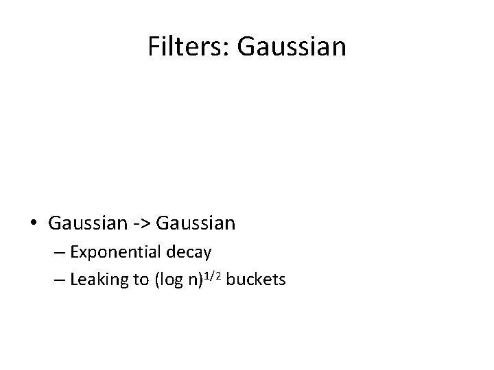
Filters: Gaussian • Gaussian -> Gaussian – Exponential decay – Leaking to (log n)1/2 buckets

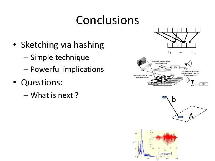
Conclusions • Sketching via hashing – Simple technique – Powerful implications c 1 … cm • Questions: – What is next ? b A